Documentation

• 1: ORCA Software-Defined Radar
• 1.1: Hardware
• 1.2: Setup Guide
• 1.2.1: Useful Commands
• 1.2.2: ORCA Setup
• 1.2.2.1: SSH
• 1.2.2.2: Git
• 1.2.3: Raspberry Pi Setup
• 1.2.3.1: Network Config
• 1.2.3.2: User Data Config
• 1.2.4: Connect and Control Options
• 1.2.5: Connecting the SDR and Testing
• 1.2.5.1: Runtime Overview
• 1.3: Radar Code
• 1.3.1: Configuration options
• 1.3.2: Host computer transport parameter tuning
• 1.4: Hardware Setup
• 1.4.1: Compatible hardware
• 1.4.2: 2 - Default Setup for the Raspberry Pi
• 1.4.3: Runtime overview
• 1.4.4: Connect and Control Options
• 1.4.5: Network Configuration
• 1.4.6: 6 - Testing Layout
• 1.4.7: 7 - Debugging: Real-Time Clocks (RTC)
• 1.5: Postprocessing
• 1.5.1: File Formats
• 1.5.2: Processing Functions
• 1.5.3: Postprocessing Notebooks
• 1.5.4: Timing and timestamping
• 2: MAPPERR Multi-frequency Radar
• 2.1: MAPPERR Core Hardware
• 2.1.1: Alternative MAPPERR Configurations
• 2.2: MAPPERR Antennas
• 2.3: Towing MAPPERR
• 3: Peregrine UAV-Borne Radar
• 3.1: Peregrine Payload
• 3.1.1: Peregrine Radar Payload Box Assembly
• 3.1.2: Data Storage Options
• 3.1.3: External button
• 3.2: 5V Power Board and Power Harnesses
• 3.3: Peregrine Radar Operating Instructions
• 3.3.1: Logger Service Setup
• 3.3.2: Radar Service Setup
• 3.4: UAV Setup
• 3.4.1: UAV Power
• 3.5: Other Resources
• 3.5.1: Sourcing Custom Parts
• 4: SORA Sled-Towed Radar
• 5:

1 - ORCA Software-Defined Radar

Code for ORCA can be found on the Github Page, which contains additional details about downloading and testing ORCA on the radios that are currently available.

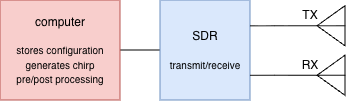
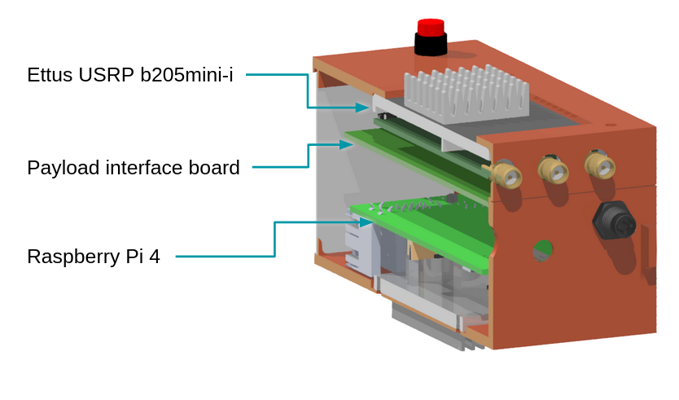
This guide is divided into three parts to help set up and understand ORCA. ORCA uses a computer and a software-defined radio (SDR) to create a functioning radar. As the architecture is currently configured, the computer is a Raspberry Pi, and the SDR is an Ettus radio. Current work is being done to implement ORCA on a Xilinx board, which would act as both a computer and SDR. Below is a simplistic block diagram that details the interaction between the hardware pieces that ORCA is intended to be used for.

1.1 - Hardware

Selecting a Software-Defined Radio (SDR)

ORCA is built upon the USRP Hardware Driver (UHD). As such, it is theoretically compatible with any Ettus SDR. We have primarily tested with B and X series devices (B205mini and X310, in particular), however most other Ettus SDRs should work with minor tweaks.

The basic capabilities of the two models we regularly use are detailed below:

In general, we recommend B series devices for applications with constraints on size, weight, power, or budget. When capabilities beyond the B series are needed, we recommend the X series.

If no device in either series suits your needs, consider other Ettus SDRs. Most should work with minor tweaks. The exception to note are E series devices, which include an embedded computer running Linux. In theory, this code could be run on that embedded computer, however the performance limitations would limit the use cases.

Host Computer

Unless you choose an E series device (see caution above), you will also need a computer to interface with the SDR. This computer is where the ORCA code will run.

The capabilities of the computer can make a significant difference in the system performance. The host computer must support an interface with enough bandwidth for the samples you want to transfer and be able to store these samples to an appropriate storage medium.

If you’re not resource constrained, a modern laptop will provide more than enough processing power, as long as it supports the interface you need. Keep in mind that X-series SDRs need a 10 gigabit ethernet (10 GigE) interface to achieve maximum sample rates. Few laptops natively support 10 GigE, however there are Thunderbolt adapters available. (Not all USB C ports support Thunderbolt and it may not be available on low-end laptops.)

For an embedded solution, Raspberry Pi’s are suitable for working with B series devices. The performance of the Raspberry Pi 5 greatly exceeds the Raspberry Pi 4, likely due to the introduction of a new USB interface chip.

Some caution is advised with other single-board computers. Their performance will likely be limited by their choice of USB controller chip.

For some examples of duty cycles achievable with various combinations of SDRs and host computers, see the figure below. Note that actual performance will depend on a variety of factors, including your exact configuration and the speed of your storage medium.

MicroSD Card

Not all (micro) SD cards are the same. Speed and reliability can both vary a lot.

Especially if you plan to store your data to your MicroSD card, you don’t want to mess around with this. Don’t use an SD card that’s off-brand, questionably sourced (i.e. possibly counterfeit), or used.

We use Samsung Pro Plus series MicroSD cards. There are other storage options too. See Other Storage Options for details.

1.2 - Setup Guide

The setup guide will include these steps:

1. Understanding which hardware to use
2. Downloading ORCA on your laptop
3. Getting your Raspberry Pi set up
4. Getting the ORCA code on the Raspberry Pi
5. Connecting to the SDR with your Raspberry Pi
6. Testing
   • Transmitter test using a spectrum analyzer
   • Receiver test using a wave and signal generator
   • Loopback test
   • Outdoor test

At the end of this process, your SDR and Raspberry Pi should be able to be used as a radar.

Beneath are links because the website puts them there, you can ignore them. They are there because they are in the level beneath the Setupguide.

1.2.1 - Useful Commands

Git

Here is also a great website to learn about git processes.

Conda

1.2.2 - ORCA Setup

The following instructions are for Windows devices. There may be different processes for different OS systems. If you find out how to set ORCA up for different devices, feel free to add to this documentation.

Creating an SSH key and connecting it to GitHub

We will create an SSH key and connecting it to your GitHub. Connecting to GitHub is technically optional but it is highly recommended. Otherwise, you have to manually type in your SSH key to add it the the Raspberry Pi which is difficult and you have a high chance of a typo.

1. Create an account on GitHub and sign in.
2. To double check that you dont already have an SSH key, open Git Bash terminal and run ls -al ~/.ssh. If you don’t already have one, it will say so. If you don’t have Git Bash already, download it here
3. We will create an SSH key now. In the Git Bash terminal, run ssh-keygen -t ed25519 -C "your-email@example.com" and accept the default location.
4. Create a password a memoriable and relatively easy to type password. You will input this every time you pull or push code to GitHub from your terminal, every time you SSH to the pi, and every time you transfer files to and from the pi. This happens a lot, so you may not want your password to be like qv34%3bj2!8ncF and 24 characters long. This however, is entirely up to you as you are the one typing the password. Additionally, please do not make your password as easy as password. A new public key file should be made.
5. Run cat ~/.ssh/id_ed25519.pub to print out the key to the terminal, and copy it. It starts with “ssh” and ends with your email. You want this whole thing. If you forget the .pub, it prints out your private key, which you do not want to give GitHub!! Do not copy out your private key!
   If that command doesn’t work, and you happen to be in the .ssh directory, you can run cat id_ed25519.pub
6. In GitHub, open settings and go to the SSH and GPG keys tab, and add a new SSH key.
7. Name this whatever you want and paste the key into the correct field.
   If you need more help with making an SSH key, here is a helpful GitHub link

SSH Agent Forwarding

After making your SSH key, you need to add it to your SSH agent on your laptop. First we need the SSH agent to be running.

1. In powershell run Get-Service -Name ssh-agent.
2. If it says the status is stopped, run Start-Service ssh-agent.
3. Run Get-Service -Name ssh-agent again and check it says the status is running.
4. To add your key, run ssh-add C:/Users/YOUR-NAME/.ssh/id_ed25519. You will need to insert the secure passphrase you made when you originally made your SSH key. It should say “Identity added”.
5. You can test this by running ssh -T git@github.com. It will say that you have been successfully authenticated, but GitHub does not provide shell access .

Installing dependencies

If you are using a Raspberry Pi, you will also want to get miniconda for the Raspberry Pi. This will be done later once the Pi is up and running. You still want to do this section so you can run the code on your laptop when making plots.

1. Install WSL (Windows Subsystem for Linux)
2. From the Start menu, open Powershell and type wsl --install.
3. Install VSCode (or some other code editor of choice).
4. If you’re using VSCode, open the Extensions tab and install the following extensions: Python, C/C++, and CMake Tools
5. Within VSCode, open a new Ubuntu (WSL) terminal.
   1. Open terminal with CTRL + ` .
   2. On the top right of the terminal section there will be name of the current terminal (likely powershell), plus sign, and a dropdown arrow.
   3. Hit the dropdown arrow and there will be an (Ubuntu WSL) option.
6. Create a username and password for the Linux system if prompted. This password is used when running Linux commands with administrator permissions (sudo).
7. You will need the Linux x86 Miniconda version, NOT WINDOWS and do not open your downloaded .sh file. Download here. You will need to click the Linux tab to access the correct download files. Save the file in your Downloads folder.
8. In the WSL terminal, change your location to be your Downloads folder.
   1. You can see your current location on the side
   2. Use cd folder-name to enter a specific folder
   3. Use cd .. to go up a folder
9. Run bash Miniconda3-latest-Linux-x86_64.sh and accept the default options in the installer (select yes when prompted about auto_activate_base, though we will change this later). Accept yes to the liscense terms. It will take time to load. If you hit enter and a new blank line appears, that means it is loading.
10. After Miniconda has been installed, close and reopen the WSL terminal. Next to the dropdown arrow where you first opened the WSL terminal is a trashcan to close the terminal.
11. To ensure it has been installed, run conda list and you should see a list of the installed dependencies printed out.
12. We are now going to change one of the default settings with the command conda config --set auto_activate_base false

Cloning the Repository

Next we will clone the GitHub repository, so it can be accessed locally.

1. Go to the ORCA repository and click the green code button and click open with github desktop
2. Click the green Code button and within the dropdown go to the SSH tab.
3. Copy the repository link which should end in .git
4. In the Git Bash terminal, navigate to whichever folder you would like the code to be copied into (with cd folder-name and/or cd ..), and run git clone link_to_repo.git.
5. In VSCode, you can now open this folder to see all the code

Setting up Conda

• We now need to use Conda to install the required dependencies for ORCA.
• Before we create the conda environment, check that GCC is installed by running gcc --version in the WSL terminal. If the gcc command is not found then install it with sudo apt update and sudo apt install gcc
• In the WSL terminal, navigate to the folder you just cloned the code to and run conda env create -f environment-rpi.yaml
• Once the environment is installed, run conda activate uhd
• Run uhd_images_downloader
• The code is now installed and ready to run or modified.

1.2.2.1 - SSH

SSH stands for secure shell. This is another way to connect to other cloud services or devices without needing to login each time. SSH is being used here with GitHub and the Raspberry Pi. You can clone a repository using SSH and you can connect to your Raspberry Pi’s terminal from your laptop using SSH.

Whenever you generate a key on your laptop, it creates both a public and private version. The public version is what you give to things like GitHub or the Raspberry Pi. The private key is what you keep on your laptop and don’t share with anyone.

Whenever you try to connect to something, like GitHub with the SSH key, something happens where the public and private key are compared and verified. Then GitHub is like cool, you’re you, and allows you to clone repositories.

To connect to your Raspberry Pi’s terminal from your laptop, you first give it the public key. After it is connected to the wifi, it is able to copy it from GitHub. Further details are in the setting up your Raspberry Pi page. Then when you try to connect to the Raspberry Pi, the two keys are compared. After verification, you then can access the Pi’s terminal. If verification fails, you can’t access the terminal.

1.2.2.2 - Git

Using Git

Git is a version control system that is used to keep track of changes to code, work on separate branches, and collaborate with other developers on the same codebase. It connects your local (offline) code to the remote (cloud) repository on GitHub. Below is basic information on how to use Git.

Cloning and pulling

To initially copy a repository from GitHub, use the git clone <repo-link> (you may need to include the https:// portion of the link or use SSH which is explained above) command as shown above. After you’ve cloned a repository, you can update your local repository with the latest version available on GitHub with the git pull command. When multiple people are working on the same branch, it is important to pull the latest code before pushing anything new.

Comitting Changes

When you have made new changes you want to push to GitHub, you will need to make a commit. First, add all the files you changed using git add -A which adds all modified files. If you only want to add a few specific ones, you can do git add file1.txt file2.txt. The terminal does need to be in the correct folder to add specific files. If the terminal is in a folder above the editted files, you can run git add ./folder/file.txt to add them. Another option is to change the terminal’s location with cd folder.

After adding files, create a new commit using git commit -m "Commit message". To make this commit available on GitHub, push the changes with git push. Git may ask you to explicitly define the upstream branch you are trying to push to, in this case follow the suggestions given such as git push -u origin branchname or git push --set-upstream origin branchname. This process is to link your local branch to a branch on the cloud. You can make multiple commits locally before pushing it to GitHub, or you can push right away after making a commit.

Branches

Git allows you to have multiple branches of the code. Each branch keeps different changes and commits, then the two branches can be merged back together. It is standard practice to make a new branch for each new feature that is being added, as it avoids problems introduced by having multiple partially implemented features conflicting with each other, as well as conflicts introduced by multiple developers working on the same file at the same time. A new branch can be created with git checkout -b branchname. Once the branch is created, you can switch between branches with git checkout branchname (the default branch is called “main”). If changes were made to the main branch after you created your branch and you want to include them in your branch, you can merge the main branch into yours. First make sure you are on your branch (git branch will tell you what branch you are on, to exit hit q), then run git fetch origin and git merge origin/main. You may run into merge conflicts which occur when each branch makes changes to the same lines of code. VS Code has a nice built-in GUI for resolving merge conflicts, which allows you to select which change to make.

VS Code also a different UI to do all of the items mentioned above instead of using a terminal if you want to search it up.

If you want to learn more. Here is a good link.

1.2.3 - Raspberry Pi Setup

In order to standardize between units, much of the Pi setup is automated or semi-automated. This guide will walk you through the steps of setting up your Pi the way we do. Along the way, there are also links for more information on how to customize this setup. This is an area where you will almost certainly need to customize some aspects of the setup.

Imaging your Pi

To start, download the Raspberry Pi Imager tool (or use your preferred software for imaging SD cards). Imaging is basically giving the Raspberry Pi an operating system. On Ubuntu, you can install it like this:

sudo apt install rpi-imager

For other operating systems, download the tool from here.

1. Launcher the imager
2. Select what version of Raspberry Pi you are using
3. Under “OS” select “Other general-purpose OS”
4. Select Ubuntu
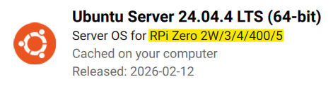
5. Scroll until you find Ubuntu Server 24.04.xx LTS (64-bit). Make sure you get 64-bit, 32-bit will not work. Also make sure that the Raspberry Pi you are using is supported.

6. Insert your SD card if you haven’t already done so, and select it
7. Skip customization, we will create our own user-data file to insert
8. Image the SD card

After imaging is complete, you should see a system-boot drive and maybe a writable drive. system-boot is more important.

Cloud-init

Setup of the Raspberry Pi is semi-automated using cloud-init.

Cloud-init customization

The cloud-init setup is controlled by two files: user-data and network-config. (You’ll use these files a couple of steps down.)

Examples of each are shown below, but you will likely need to modify these to suit your purpose. We have pages on how to customize network-config and user-data. If you are trying to connect to an enterprise Wi-Fi like a university’s guest wifi, maybe you need to contact OIT to get your device whitelisted. This is how it is at CU Boulder, and I have no idea about how other university’s Wi-Fis work.

user-data Example

#cloud-config

# This is the user-data configuration file for cloud-init.
# The cloud-init documentation has more details:
#
# https://cloudinit.readthedocs.io/

system_info:
  default_user:
    name: ubuntu # Allow the default user to shutdown or reboot the system without entering a password (used by our automated scripts)
    sudo: "ALL=(ALL) NOPASSWD: /sbin/poweroff, /sbin/reboot, /sbin/shutdown"

# On first boot, set the (default) ubuntu user's password to "cryosphere"
chpasswd:
  expire: false
  users:
    - name: ubuntu
      password: $6$rounds=4096$aQ7tu0.beL3WAL32$fKxKYvZpY7EMCoxAU1heRomA3v8WvgbqBhhz08QwOtQdlP/DJOP2BThqZFoRW8d2a9PaIKK9BC9NHs1qNnkya1
      type: hash

# Enable password authentication with the SSH daemon
ssh_pwauth: true

# Set a default timezone
timezone: Etc/UTC

## Update apt database and upgrade packages on first boot
package_update: true
package_upgrade: true

## Install additional packages on first boot
packages:
- net-tools
- git
- cmake
- g++
- mosh
- exfat-fuse
- i2c-tools
- rpi.gpio-common
- util-linux-extra
- gpsd
- gpsd-clients

## Write arbitrary files to the file-system
write_files:
- path: /home/ubuntu/initial_setup.sh
  content: |
    #!/bin/bash
    exec > >(tee -a "initial_setup_output.log") 2>&1
    # Miniconda Setup
    wget --progress=bar:force:noscroll "https://github.com/conda-forge/miniforge/releases/latest/download/Miniforge3-Linux-aarch64.sh" -O $HOME/miniconda.sh
    bash $HOME/miniconda.sh -b -p $HOME/miniconda
    cd $HOME
    source .profile
    source miniconda/etc/profile.d/conda.sh
    conda init bash
    # Setup logger environment
    git clone git@github.com:thomasteisberg/uav_radar_logger.git
    # Clone uhd_radar repo
    git clone git@github.com:radioglaciology/uhd_radar.git
    cd uhd_radar
    #git checkout thomas/dask # Uncomment if you want to check out a specific branch other than main
    conda env create -n uhd -f environment-rpi.yaml
    conda activate uhd
    python /home/ubuntu/miniconda/envs/uhd/lib/uhd/utils/uhd_images_downloader.py
    systemctl --user enable radar.service
    systemctl --user enable logger.service
    ifconfig
    sudo reboot
  append: true
- path: /home/ubuntu/.profile
  content: |
    PATH=/home/ubuntu/miniconda/bin:$PATH
    source /home/ubuntu/.bashrc
  append: true
- path: /home/ubuntu/.ssh/known_hosts
  content: |
    github.com ssh-ed25519 AAAAC3NzaC1lZDI1NTE5AAAAIOMqqnkVzrm0SdG6UOoqKLsabgH5C9okWi0dh2l9GKJl
    github.com ecdsa-sha2-nistp256 AAAAE2VjZHNhLXNoYTItbmlzdHAyNTYAAAAIbmlzdHAyNTYAAABBBEmKSENjQEezOmxkZMy7opKgwFB9nkt5YRrYMjNuG5N87uRgg6CLrbo5wAdT/y6v0mKV0U2w0WZ2YB/++Tpockg=
    github.com ssh-rsa AAAAB3NzaC1yc2EAAAADAQABAAABgQCj7ndNxQowgcQnjshcLrqPEiiphnt+VTTvDP6mHBL9j1aNUkY4Ue1gvwnGLVlOhGeYrnZaMgRK6+PKCUXaDbC7qtbW8gIkhL7aGCsOr/C56SJMy/BCZfxd1nWzAOxSDPgVsmerOBYfNqltV9/hWCqBywINIR+5dIg6JTJ72pcEpEjcYgXkE2YEFXV1JHnsKgbLWNlhScqb2UmyRkQyytRLtL+38TGxkxCflmO+5Z8CSSNY7GidjMIZ7Q4zMjA2n1nGrlTDkzwDCsw+wqFPGQA179cnfGWOWRVruj16z6XyvxvjJwbz0wQZ75XK5tKSb7FNyeIEs4TT4jk+S4dhPeAUC5y+bDYirYgM4GC7uEnztnZyaVWQ7B381AK4Qdrwt51ZqExKbQpTUNn+EjqoTwvqNj4kqx5QUCI0ThS/YkOxJCXmPUWZbhjpCg56i+2aB6CmK2JGhn57K5mj0MNdBXA4/WnwH6XoPWJzK5Nyu2zB3nAZp+S5hpQs+p1vN1/wsjk=
- path: /etc/security/limits.conf # Recommended by Ettus https://kb.ettus.com/USRP_Host_Performance_Tuning_Tips_and_Tricks
  content: |
    ubuntu    - rtprio    99
  append: true
- path: /etc/systemd/user/radar.service
  content: |
    [Unit]
    Description=Service to run the radar code on startup

    [Service]
    Type=simple
    WorkingDirectory=/home/ubuntu/uhd_radar/
    ExecStart=/home/ubuntu/uhd_radar/manager/radar_service.sh

    Restart=always
    RestartSec=10

    KillSignal=SIGINT

    [Install]
    WantedBy=default.target
- path: /etc/systemd/user/logger.service
  content: |
    [Unit]
    Description=Service to log data from I2C sensors and automatically shutdown below a voltage threshold

    [Service]
    Type=simple
    WorkingDirectory=/home/ubuntu/uav_radar_logger/
    ExecStart=/home/ubuntu/uav_radar_logger/logger_service.sh

    Restart=always
    RestartSec=60

    KillSignal=SIGINT

    [Install]
    WantedBy=default.target

# Run arbitrary commands at rc.local like time
# These commands are run with root permissions
# If you want commands run as a normal user, put them in initial_setup.sh (see above)
# which is run as the "ubuntu" user (see below)
runcmd:
- chown -R ubuntu:ubuntu /home/ubuntu
- chmod +x /home/ubuntu/initial_setup.sh
- wget -O /etc/udev/rules.d/uhd-usrp.rules https://raw.githubusercontent.com/EttusResearch/uhd/master/host/utils/uhd-usrp.rules
- usermod -a -G i2c ubuntu
- usermod -a -G dialout ubuntu
- usermod -a -G tty ubuntu
- apt remove -y modemmanager
- systemctl stop serial-getty@ttyS0.service && systemctl disable serial-getty@ttyS0.service
- i2cdetect -y 1
- echo "dtoverlay=i2c-rtc,pcf8523" >> /boot/firmware/config.txt
- loginctl enable-linger ubuntu
- mkdir /media/ssd
- chown ubuntu /media/ssd
- chgrp ubuntu /media/ssd
- echo "/dev/sda2  /media/ssd  exfat  defaults,nofail,uid=1000,gid=1000  0  2" | tee -a /etc/fstab

network-config Example

# This file contains a netplan-compatible configuration which cloud-init will
# apply on first-boot (note: it will *not* update the config after the first
# boot). Please refer to the cloud-init documentation and the netplan reference
# for full details:
#
# https://cloudinit.readthedocs.io/en/latest/topics/network-config.html
# https://cloudinit.readthedocs.io/en/latest/topics/network-config-format-v2.html
# https://netplan.io/reference

version: 2
ethernets:
  eth0:  # Your ethernet name.
    dhcp4: no
    addresses: [192.168.11.137/24]
    gateway4: 192.168.11.1
    nameservers:
      addresses: [8.8.8.8,8.8.4.4]
wifis:
  renderer: networkd
  wlan0:
    dhcp4: true
    optional: true
    access-points:
      "<YOUR WIFI SSID HERE>":
        password: "<YOUR WIFI PASSWORD HERE>"

network-config Example for Laptop Mobile Hotspot and Possibly Normal Wifi

# This file contains a netplan-compatible configuration which cloud-init will
# apply on first-boot (note: it will *not* update the config after the first
# boot). Please refer to the cloud-init documentation and the netplan reference
# for full details:
#
# https://cloudinit.readthedocs.io/en/latest/topics/network-config.html
# https://cloudinit.readthedocs.io/en/latest/topics/network-config-format-v2.html
# https://netplan.io/reference

network:
  version: 2
  renderer: networkd
  wifis:
    wlan0:
      dhcp4: yes
      access-points:
        "<WIFI SSID HERE>":
          password: "<PASSWORD HERE>"

After you edit the user-data and network-config files and add them to your SD card. You can now put the card back into the Pi.

1.2.3.1 - Network Config

Setting up network interfaces

With cloud-init (first-time setup)

The preferred way to setup network interfaces is by providing them in the network-config file read by cloud-init when first setting up the Pi.

An example is shown below:

# This file contains a netplan-compatible configuration which cloud-init will
# apply on first-boot (note: it will *not* update the config after the first
# boot). Please refer to the cloud-init documentation and the netplan reference
# for full details:
#
# https://cloudinit.readthedocs.io/en/latest/topics/network-config.html
# https://cloudinit.readthedocs.io/en/latest/topics/network-config-format-v2.html
# https://netplan.io/reference

version: 2
ethernets:
  eth0:  # Your ethernet name.
    dhcp4: no
    addresses: [192.168.11.137/24]
    gateway4: 192.168.11.1
    nameservers:
      addresses: [8.8.8.8,8.8.4.4]
wifis:
  renderer: networkd
  wlan0:
    dhcp4: true
    optional: true
    access-points:
      "<YOUR WIFI SSID HERE>":
        password: "<YOUR WIFI PASSWORD HERE>"

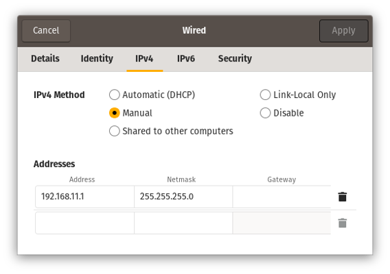
The above configuration sets up a static IP over the ethernet interface. It also configures 192.168.11.1 as the default gateway. This allows for sharing an internet connection from a computer over this interface if desired.

The configuration also provides an SSID and password for a WiFi network. In practice, we configure this to the settings for a phone hotspot that can be used to get internet when WiFi is not otherwise available. This is also a simpler setup for getting the Pi on the internet when needed.

Reconfiguring with netplan

By default, network interfaces are configured with netplan. See the netplan documentation for more details.

By default, the cloud-init script sets up a static IP of 192.168.11.137, but you could choose to configure this to something different for each payload box.

Our usual way of connecting is by plugging an ethernet cable into the Pi and connecting it to a laptop. You can read about all the networking options here.

1.2.3.2 - User Data Config

Use this when setting up your Raspberry Pi on initial boot-up.

The default user-data we start from is as shown below. You will likely need to tweak many of these settings. Descriptions and tips for the most important sections are below.

Note that this is one of two key configuration files. You can read about network-config here.

Starting point user-data file

#cloud-config

# This is the user-data configuration file for cloud-init.
# The cloud-init documentation has more details:
#
# https://cloudinit.readthedocs.io/

system_info:
  default_user:
    name: ubuntu # Allow the default user to shutdown or reboot the system without entering a password (used by our automated scripts)
    sudo: "ALL=(ALL) NOPASSWD: /sbin/poweroff, /sbin/reboot, /sbin/shutdown"

# On first boot, set the (default) ubuntu user's password to "cryosphere"
chpasswd:
  expire: false
  users:
    - name: ubuntu
      password: $6$rounds=4096$aQ7tu0.beL3WAL32$fKxKYvZpY7EMCoxAU1heRomA3v8WvgbqBhhz08QwOtQdlP/DJOP2BThqZFoRW8d2a9PaIKK9BC9NHs1qNnkya1
      type: hash

# Enable password authentication with the SSH daemon
ssh_pwauth: true

# Set a default timezone
timezone: Etc/UTC

## Update apt database and upgrade packages on first boot
package_update: true
package_upgrade: true

## Install additional packages on first boot
packages:
- net-tools
- git
- cmake
- g++
- mosh
- exfat-fuse
- i2c-tools
- rpi.gpio-common
- util-linux-extra
- gpsd
- gpsd-clients

## Write arbitrary files to the file-system
write_files:
- path: /home/ubuntu/initial_setup.sh
  content: |
    #!/bin/bash
    exec > >(tee -a "initial_setup_output.log") 2>&1
    # Miniconda Setup
    wget --progress=bar:force:noscroll "https://github.com/conda-forge/miniforge/releases/latest/download/Miniforge3-Linux-aarch64.sh" -O $HOME/miniconda.sh
    bash $HOME/miniconda.sh -b -p $HOME/miniconda
    cd $HOME
    source .profile
    source miniconda/etc/profile.d/conda.sh
    conda init bash
    # Setup logger environment
    git clone git@github.com:thomasteisberg/uav_radar_logger.git
    # Clone uhd_radar repo
    git clone git@github.com:radioglaciology/uhd_radar.git
    cd uhd_radar
    #git checkout thomas/dask # Uncomment if you want to check out a specific branch other than main
    conda env create -n uhd -f environment-rpi.yaml
    conda activate uhd
    python /home/ubuntu/miniconda/envs/uhd/lib/uhd/utils/uhd_images_downloader.py
    systemctl --user enable radar.service
    systemctl --user enable logger.service
    ifconfig
    sudo reboot
  append: true
- path: /home/ubuntu/.profile
  content: |
    PATH=/home/ubuntu/miniconda/bin:$PATH
    source /home/ubuntu/.bashrc
  append: true
- path: /home/ubuntu/.ssh/known_hosts
  content: |
    github.com ssh-ed25519 AAAAC3NzaC1lZDI1NTE5AAAAIOMqqnkVzrm0SdG6UOoqKLsabgH5C9okWi0dh2l9GKJl
    github.com ecdsa-sha2-nistp256 AAAAE2VjZHNhLXNoYTItbmlzdHAyNTYAAAAIbmlzdHAyNTYAAABBBEmKSENjQEezOmxkZMy7opKgwFB9nkt5YRrYMjNuG5N87uRgg6CLrbo5wAdT/y6v0mKV0U2w0WZ2YB/++Tpockg=
    github.com ssh-rsa AAAAB3NzaC1yc2EAAAADAQABAAABgQCj7ndNxQowgcQnjshcLrqPEiiphnt+VTTvDP6mHBL9j1aNUkY4Ue1gvwnGLVlOhGeYrnZaMgRK6+PKCUXaDbC7qtbW8gIkhL7aGCsOr/C56SJMy/BCZfxd1nWzAOxSDPgVsmerOBYfNqltV9/hWCqBywINIR+5dIg6JTJ72pcEpEjcYgXkE2YEFXV1JHnsKgbLWNlhScqb2UmyRkQyytRLtL+38TGxkxCflmO+5Z8CSSNY7GidjMIZ7Q4zMjA2n1nGrlTDkzwDCsw+wqFPGQA179cnfGWOWRVruj16z6XyvxvjJwbz0wQZ75XK5tKSb7FNyeIEs4TT4jk+S4dhPeAUC5y+bDYirYgM4GC7uEnztnZyaVWQ7B381AK4Qdrwt51ZqExKbQpTUNn+EjqoTwvqNj4kqx5QUCI0ThS/YkOxJCXmPUWZbhjpCg56i+2aB6CmK2JGhn57K5mj0MNdBXA4/WnwH6XoPWJzK5Nyu2zB3nAZp+S5hpQs+p1vN1/wsjk=
- path: /etc/security/limits.conf # Recommended by Ettus https://kb.ettus.com/USRP_Host_Performance_Tuning_Tips_and_Tricks
  content: |
    ubuntu    - rtprio    99
  append: true
- path: /etc/systemd/user/radar.service
  content: |
    [Unit]
    Description=Service to run the radar code on startup

    [Service]
    Type=simple
    WorkingDirectory=/home/ubuntu/uhd_radar/
    ExecStart=/home/ubuntu/uhd_radar/manager/radar_service.sh

    Restart=always
    RestartSec=10

    KillSignal=SIGINT

    [Install]
    WantedBy=default.target
- path: /etc/systemd/user/logger.service
  content: |
    [Unit]
    Description=Service to log data from I2C sensors and automatically shutdown below a voltage threshold

    [Service]
    Type=simple
    WorkingDirectory=/home/ubuntu/uav_radar_logger/
    ExecStart=/home/ubuntu/uav_radar_logger/logger_service.sh

    Restart=always
    RestartSec=60

    KillSignal=SIGINT

    [Install]
    WantedBy=default.target

# Run arbitrary commands at rc.local like time
# These commands are run with root permissions
# If you want commands run as a normal user, put them in initial_setup.sh (see above)
# which is run as the "ubuntu" user (see below)
runcmd:
- chown -R ubuntu:ubuntu /home/ubuntu
- chmod +x /home/ubuntu/initial_setup.sh
- wget -O /etc/udev/rules.d/uhd-usrp.rules https://raw.githubusercontent.com/EttusResearch/uhd/master/host/utils/uhd-usrp.rules
- usermod -a -G i2c ubuntu
- usermod -a -G dialout ubuntu
- usermod -a -G tty ubuntu
- apt remove -y modemmanager
- systemctl stop serial-getty@ttyS0.service && systemctl disable serial-getty@ttyS0.service
- i2cdetect -y 1
- echo "dtoverlay=i2c-rtc,pcf8523" >> /boot/firmware/config.txt
- loginctl enable-linger ubuntu
- mkdir /media/ssd
- chown ubuntu /media/ssd
- chgrp ubuntu /media/ssd
- echo "/dev/sda2  /media/ssd  exfat  defaults,nofail,uid=1000,gid=1000  0  2" | tee -a /etc/fstab

Password-less shutdown

system_info:
  default_user:
    name: ubuntu # Allow the default user to shutdown or reboot the system without entering a password (used by our automated scripts)
    sudo: "ALL=(ALL) NOPASSWD: /sbin/poweroff, /sbin/reboot, /sbin/shutdown"

One of the features supported by the uav_radar_logger utility is to automatically cleanly shutdown the system if the measured battery voltage drops below a threshold. To facilitate this, the default user must be able to shutdown the system without needing additional authentication. This gives permission for the ubuntu user to call sudo shutdown or sudo reboot without entering a password.

Password authentication

# On first boot, set the (default) ubuntu user's password to "cryosphere"
chpasswd:
  expire: false
  list:
  - ubuntu:$6$rounds=4096$aQ7tu0.beL3WAL32$fKxKYvZpY7EMCoxAU1heRomA3v8WvgbqBhhz08QwOtQdlP/DJOP2BThqZFoRW8d2a9PaIKK9BC9NHs1qNnkya1

# Enable password authentication with the SSH daemon
ssh_pwauth: true

This sets up a default password for the ubuntu user. You should change this to something else (or disable password authentication completely, if you prefer).

Passwords are stored in a hashed format. You can generate password hashes using this utility:

mkpasswd --method=SHA-512 --rounds=4096

Timezone

# Set a default timezone
timezone: Etc/UTC

You could set this to other time zones (i.e. `America/Los_Angeles"), but really it would make everyone’s life easier if you just set your clock to UTC.

Add SSH keys through GitHub

## On first boot, use ssh-import-id to give the specific users SSH access to
## the default user
ssh_import_id:
- gh:thomasteisberg
- gh:albroome
- gh:dfxmay

You can very conveniently enable key-based authentication for specific GitHub user names. If your username is in here and you have a public key setup with GitHub, this public key will be imported and you will be able to SSH into your Pi with no additional setup. You might want to remove us from your list, though. :)

Files

Arbitrary files can be written to the system with cloud-init. Some of these are important.

initial_setup.sh

- path: /home/ubuntu/initial_setup.sh
  content: |
    #!/bin/bash
    exec > >(tee -a "initial_setup_output.log") 2>&1
    # Miniconda Setup
    wget --progress=bar:force:noscroll "https://github.com/conda-forge/miniforge/releases/latest/download/Miniforge3-Linux-aarch64.sh" -O $HOME/miniconda.sh
    bash $HOME/miniconda.sh -b -p $HOME/miniconda
    cd $HOME
    source .profile
    source miniconda/etc/profile.d/conda.sh
    conda init bash
    # Setup logger environment
    git clone git@github.com:thomasteisberg/uav_radar_logger.git
    # Clone uhd_radar repo
    git clone git@github.com:radioglaciology/uhd_radar.git
    cd uhd_radar
    #git checkout thomas/dask # Uncomment if you want to check out a specific branch other than main
    conda env create -n uhd -f environment.yaml
    conda activate uhd
    python /home/ubuntu/miniconda/envs/uhd/lib/uhd/utils/uhd_images_downloader.py
    systemctl --user enable radar.service
    systemctl --user enable logger.service
    ifconfig
    sudo reboot
  append: true

The initial_setup.sh script grabs copies of our code and sets up the radar and logging services. This script is intended to be manually run the first time you SSH into the system. This enables you to use SSH agent forwarding to provide any needed GitHub authentication to get the code.

This is also where you would customize the repositories to check out (if, for example, you’ve forked our code) and where you can pick a branch to automatically checkout.

Radar and Logger services

- path: /etc/systemd/user/radar.service
  content: |
    [Unit]
    Description=Service to run the radar code on startup

    [Service]
    Type=simple
    WorkingDirectory=/home/ubuntu/uhd_radar/
    ExecStart=/home/ubuntu/uhd_radar/manager/radar_service.sh

    Restart=always
    RestartSec=10

    KillSignal=SIGINT

    [Install]
    WantedBy=default.target
- path: /etc/systemd/user/logger.service
  content: |
    [Unit]
    Description=Service to log data from I2C sensors and automatically shutdown below a voltage threshold

    [Service]
    Type=simple
    WorkingDirectory=/home/ubuntu/uav_radar_logger/
    ExecStart=/home/ubuntu/uav_radar_logger/logger_service.sh

    Restart=always
    RestartSec=60

    KillSignal=SIGINT

    [Install]
    WantedBy=default.target

Two systemd services are used to manage everything. One run the radar code in its default button-controlled setup. The other runs basic logging of I2C-connected sensors and handles automatic low-battery shutdown.

Run commands

runcmd:
- chown -R ubuntu:ubuntu /home/ubuntu
- chmod +x /home/ubuntu/initial_setup.sh
- wget -O /etc/udev/rules.d/uhd-usrp.rules https://raw.githubusercontent.com/EttusResearch/uhd/master/host/utils/uhd-usrp.rules
- usermod -a -G i2c ubuntu
- usermod -a -G dialout ubuntu
- usermod -a -G tty ubuntu
- apt remove -y modemmanager
- systemctl stop serial-getty@ttyS0.service && systemctl disable serial-getty@ttyS0.service
- i2cdetect -y 1
- echo "dtoverlay=i2c-rtc,pcf8523" >> /boot/firmware/config.txt
- loginctl enable-linger ubuntu
- mkdir /media/ssd
- echo "/dev/sda2  /media/ssd  exfat  defaults,nofail,uid=1000,gid=1000  0  2" | tee -a /etc/fstab

Some final setup is done by running arbitrary commands. These are run as the root user.

One aspect of this you may wish to customize are the last two lines, which add settings to automatically mount an ExFAT-formatted SSD plugged into the Pi. This can be (optionally) used as a storage location for radar data.

Testing changes

You may want to test your changes before using them on your Pi. Options for doing that are described here. Note that the initial_setup.sh script downloads miniconda for the aarch64 architecture, which probably won’t work on your computer. If you want to test that part, you’ll need to change this.

1.2.4 - Connect and Control Options

Connecting to the Pi

We will be using SSH to connect your laptop to the Pi. You can do this either over wifi or ethernet. Before doing this, we need to get the IP address of the Pi and import your public SSH key onto the Pi.

Direct Control

This is the process to get the IP address of the Pi and import your public SSH key.

This method requires a monitor and keyboard, cannot be used to share files between a laptop and the Pi, and is more difficult to use. However, we need to use this, mainly to import your SSH key. This is also useful in case the network-config isn’t working. Direct control allows you to edit the file that controls this.

To access the Pi’s terminal directly you will need:

• Raspberry Pi 5
• Pi Power Supply (plugged into wall)
• Monitor (plugged into wall)
• HDMI to Micro-HDMI cable
• Keyboard
• Ethernet cable connected to a router (or ethernet port on the wall of the lab) or just connect the Pi to wifi

Simply connect the ethernet (or just use WiFi), micro-HDMI, keyboard, and power supply to the Raspberry Pi. When it boots, you will see the cloud-init running a bunch of things and the Pi’s Ubuntu Server terminal on the monitor.

Running Cloud-init

Power up the Pi and wait for cloud-init to run.

Within about a minute, your Pi should connect to whatever network interface(s) are described in network-config and you should be able to find it on the network. If you setup some sort of key-based authentication (such as by importing a key from GitHub), it may take an extra couple of minutes for this to be ready.

After the network setup is complete, you should be able to login over SSH if you edited the user-data file to import your SSH key. However if that process failed, then you’ll have to manually import your SSH key.

In particular, please note that you need to have SSH agent forwarding working on your laptop. You should have already done this under ORCA Setup when you first made your SSH key. You can test that everything is working by running ssh -T git@github.com on your laptop.

When you first login to the Pi, cloud-init may not have finished running. To check the status, run:

cloud-init status --long

There are also logs in /var/log/cloud-init-output.log (you can read with cat or less).

To keep an eye on the entire process, you can run:

watch "cloud-init status --long && tail -n 10 /var/log/cloud-init-output.log"

Expect this process to take a few minutes to complete.

Initial Setup

When you are able to start running commands, run ./initial_setup.sh. This will log to /home/ubuntu/initial_setup_output.log. It may take around 10 minutes to complete. It will automatically reboot your Pi at the end. If you don’t want this, feel free to comment out the last line. If you don’t know where this line is, it is fine to just leave it to reboot.

After this process finishes running, run ping 8.8.8.8 to test if it is connected to wifi/ethernet. If the Pi isn’t connected, it will say “Network is unreachable”. If the Pi is connected, it will start detecting bytes sent by the address. Hit CTRL + C to stop the pinging. It will then give you a report of how much loss there was. You want to have 0 loss.

You can log in and run commands directly with the keyboard (no mouse inputs). There is no way to scroll up through this terminal however, so if you want to be able to read a long output from a command you must pipe it into a file (ex. python run.py >> terminal_output.txt), then read the text file using nano.

Importing Your SSH Key

You then need to add this SSH to the Pi. The simplest method is to first add the key to your GitHub account, then import it onto the Pi from there. If you don’t want to set up GitHub, you can add the key directly with a little extra work (though you may have typos which can make it difficult!).

With GitHub:

1. You should have already added the SSH key to your GitHub account.
2. Run ssh-import-id gh:<your-github-username> on the Raspberry Pi with the direct control.

If you haven’t yet added your key to GitHub, do the following:

1. Create an account on GitHub and sign in.
2. In GitHub, open settings and go to the SSH and GPG keys tab and add a new SSH key.
3. Name this key whatever you want and paste the key into the correct field.
4. Log into the Pi using the direct control method above.
5. Run ssh-import-id gh:<your-github-username>.

Without GitHub:

1. Log into the Pi using the direct control method above.
2. Open the authorized keys file with sudo nano ~/.ssh/authorized_keys.
3. Manually copy your key (starts with ssh-ed25519, ends with your email) into the file
4. Hit Ctrl+X followed by Y, then Enter to save the changes.

You should now have permission to SSH into the Pi from your laptop using one of the following methods (wifi or ethernet).

Modify your ~/.ssh/config file (use nano ~/.ssh/config) and add an entry like this enabling SSH agent forwarding (or don’t, you likely already set up SSH agent forwarding on your laptop so I don’t think you need to do this. I didn’t do this and it worked fine for me):

Host 192.168.11.137
    HostName 192.168.11.137
    User ubuntu
    ForwardAgent yes

Note that if your username or host IP address is different, you should adjust it accordingly.

@@@@@@@@@@@@@@@@@@@@@@@@@@@@@@@@@@@@@@@@@@@@@@@@@@@@@@@@@@@
@    WARNING: REMOTE HOST IDENTIFICATION HAS CHANGED!     @
@@@@@@@@@@@@@@@@@@@@@@@@@@@@@@@@@@@@@@@@@@@@@@@@@@@@@@@@@@@
IT IS POSSIBLE THAT SOMEONE IS DOING SOMETHING NASTY!
Someone could be eavesdropping on you right now (man-in-the-middle attack)!
It is also possible that a host key has just been changed.

ssh-keyscan -H 192.168.11.137 >> ~/.ssh/known_hosts

SSH over Ethernet:

This is a good method because the Pi is not required to be connected to a router or Wi-Fi network. However, it does take a bit of setup the first time. This method can be good if you are outside with no access to internet. There is also the SSH over Hotspot method which is also good when you are outside and you won’t need ethernet cables.

For this method, you will need:

• Laptop connected to Wi-Fi
• Raspberry Pi 5
• Pi Power Supply (plugged into wall)
• Ethernet cable
• Ethernet to usb-c adapter (if your laptop doesn’t have an ethernet port)

1. Plug the power supply into the Pi and plug one end of the ethernet cable into the Pi, and the other into your laptop.

2. Connect your laptop to any Wi-Fi network.

3. If your laptop’s public SSH key is not already on the Pi, see the section above for how to add it. (Using direct connect)

4. If this is your first time setting up this method, you will now need to enable internet sharing on your laptop. If you have done this before, then skip this step.

   • a. Windows:

     • i. Open Control Panel and go to the Network section.
     • ii. Find the Wi-Fi connection and right click on it, then go to Properties.
     • iii. At the top, click on the Sharing tab.
     • iv. Check “Allow other network users to connect…”
     • v. In the dropdown, select “Ethernet2” (not the ethernet for WSL).
     • vi. Apply the changes.

   • b. Linux:

     • i. Install Network Manager Command-line Interface (nmcli) with sudo apt install network-manager .
     • ii. Find the connection name with nmcli con show . Find the entry with type ethernet, it should have a name like “Wired connection 1”.
     • iii. Run nmcli con modify “Wired connection 1” ipv4.method shared .

5. If you are on Linux, run nmcli con up “Wired connection 1”

6. Find the Pi’s IP address on your local subnet.

   • a. If you are on Windows, open PowerShell and run arp -a. You should see an interface for 192.168.137.1 and within that section should be an IP address that starts with 192.168.137 and ends with something other than .0 or .1 (ex. 192.168.137.27).
   • b. If you are on Linux, then Pi #1 always has the IP 10.42.0.10, and Pi #2 always has the IP 10.42.0.20. If for some reason you cannot find the IP, confirm the subnet is 10.42.0 by running ip a . Under the enxc… section should say “state UP” and you should see “inet 10.42.0.1/24”. You can then scan the subnet to find the pi by running nmap -sn 10.42.0.1/24 and looking for a device that’s not 10.42.0.1. You may need to restart the Pi and give it a minute to boot.

7. Run ssh ubuntu@<pi-ip-address> to connect to the Pi. You can now run commands on the Pi, and transfer files to and from your laptop using SCP (will be explained below).

SSH over Wi-Fi:

This method is nice as it requires less cables and can be used for connecting multiple devices, however you will have to use one of the other methods such as SSH over Ethernet initially to find the Pi’s internet IP address.

For this method, you will need:

• Laptop connected to Wi-Fi
• Raspberry Pi 5
• Pi Power Supply (plugged into wall)
• Ethernet cable connected to a router (or to the ethernet port on the wall of the lab) if not connecting the Pi to Wi-Fi

1. Plug the ethernet and power cable into the Pi and turn it on. Or if the Pi is connected to Wi-Fi just leave it as is.
2. If you do not know what the Pi’s current IP address is, you must first use the Direct Control method above to get access to the terminal. You can run hostname -I and it will print out the IP address. Another way is when the Pi first boots, system information is printed to the terminal. In the bottom right corner of this message, you should see a section that says “IPv4 address for eth0 (or wlan0): 128.138.189.xxx”. You can also find the IP address by running ip a and looking for the address under the eth0 (or wlan0). This address may change each time the Pi is reconnected to the internet. This means you will consistently need direct control to see the IP address unless you set a static IP address. Information on how to do this is below.
3. Connect your laptop to a wifi network.
4. Check if you can find the Pi over the internet by running the command ping -c 1 your.pi.ip.address. On Windows, this must be done in PowerShell with admin privileges, not WSL. If it says 0 packets received, then either the IP address is incorrect, or you are not on the same network as the Pi.
5. If your laptop’s public SSH key is not already on the Pi, see the section above (Importing Your SSH Key section) for how to add it.
6. Run ssh ubuntu@your.pi.ip.address to connect to the Pi. If you chose a different login username, replace ubuntu with that. You can now run commands on the Pi, and transfer files to and from your laptop using SCP (see below).

SSH Over Hotspot:

This method is good for the outdoors where there is no Wifi/internet connection. It allows you to SSH into the Pi without internet connection, similar to SSH over ethernet, but you also won’t need an ethernet cable. If you use this method, the Pi will not be able to access a Wi-Fi internet connection at the same time, so you won’t be able to clone the repository or pull from the repository. This setup will require direct control, but afterwards you won’t need direct control again.

For this method, you will need:

• Laptop
• Raspberry Pi 5
• USB keyboard connected to the Pi (direct control)
• Monitor connected to the Pi (direct control)
• Pi Power supply

1. This method uses NetworkManager and your Pi’s connections need to be controlled with NetworkManager. Check if your netplan’s renderer is NetworkManager, if not, change it to NetworkManager.
   1. Run ls /etc/netplan/. It should show a .yaml.
   2. Run sudo nano /etc/netplan/FILENAME.yaml. This allows you to open and edit the file.
   3. Change whatever you need to, then hit CTRL + X, then y, then hit enter. This saves your edits.
   4. Run sudo netplan apply to apply these changes
   5. Try ping 8.8.8.8 again to see if is connected now. Hit Ctrl + C to stop the pinging and check that there is no packet loss.
   6. You may need to run sudo reboot
2. Run sudo apt update and sudo apt update -y
3. Run iwconfig to see the names for the different connection tools. We want the wifi one which is commonly wlan0 but it may not be the same for your Pi. It will be the one with information of IEEE and ESSID
4. DEVICE is the name of the wifi device (commonly wlan0). SSID is the name of the broadcast of the Pi. It will be what your laptop connects to. PASSWORD is the password for the connection. Run sudo nmcli d wifi hotspot ifname DEVICE ssid SSID password PASSWORD
5. You can check that it has been created by running nmcli connection show. It will look something like this

NAME                UUID                                  TYPE      DEVICE
Hotspot             59f9160c-b49f-47a2-ac54-87987f743df2  wifi      wlan0
Wired connection 1  9d27eb3e-7657-3a54-ad8a-344cb4bb56e3  ethernet  eth0
lo                  a54edcc4-0ffa-4090-a2b3-081905aee1c5  loopback  lo
preconfigured       6e07c33c-9764-4145-af3f-49875c8a9342  wifi      --

If you are connected to wifi, you will see that at the top with the wlan0 device while Hotspot’s device will be blank.

6. To swap to the Hotspot run nmcli connection up "Hotspot" and to swap back to your wifi replace Hotspot with whatever the name is for your wifi connection. While swapping connections the Pi may freak out and print an error along the lines of brcmfmac: brcmf_set_channel: set chanspec fail, reason -52. This happens whenever the Pi loses connection and isn’t a big issue.
7. If the putting the hotspot up fails with an error of Connection: activation failed: IP configuration could not be reserved try the following steps
   1. Run sudo nmcli connection modify "Hotspot" ipv4.method shared
   2. Run sudo systemctl stop dnsmasq
   3. Run sudo systemctl restart NetworkManager
   4. Run sudo nmcli connection up "Hotspot"
   5. If this works now, the problem is likely dnsmasq so we need to turn it off permenantly so it won’t turn back on and break the Hotspot when you reboot the Pi.
   6. Run sudo systemctl disable dnsmasq
   7. Run sudo systemctl mask dnsmasq
   8. Run sudo reboot
   9. Now if you run systemctl status dnsmasq it should say that it inactive (dead)
8. Since you rebooted the Pi, you may need to turn on the hotspot again with nmcli connection up "Hotspot". It should say succesfully activated and you should see the Pi’s hotspot when you open your wifi connections on your laptop. You can now connect to this.
9. Run ipconfig on your laptop’s powershell after connecting (may be a different command if not on a windows device) and look at the IP address after Default Gateway under the Wi-Fi section. This is the IP address of the PI.
10. Run ssh ubuntu@your.pi.ip.address to SSH into the Pi.

The next steps are optional but makes it so your Hotspot will be the default connection your Pi does. This makes it so if you are outside and need to connect to the Pi, you can do so immediately without needed direct control to swap the network connection from wifi to the hotspot. The default connection for the Pi seems to be Wi-Fi.

11. Run sudo nmcli connection modify "Hotspot" connection.autoconnect true
12. Run sudo nmcli connection modify "Hotspot" connection.autoconnect-priority 100
13. Run sudo nmcli connection modify "wifi connection" connection.autoconnect-priority 10 Rename “wifi connection” to whatever the name of your wifi connection is. You can check what it is with nmcli connection show. The first autoconnect priority is the higher number.

Now if you reboot the Pi, it will automatically open the hotspot first.

Setting Static IP Addresses

Setting a static IP address makes it very convenient because you won’t need to use direct control to see the Pi’s IP address everytime you want to SSH into it.

Setting a static IP address when the Pi connects to wifi

1. Run hostname -I to show your current IP. You can use the same one or don’t.
2. Run ip r | grep default and check the IP that is after the word via. That is your default gateway.
3. Run nmcli connection show to find the name of your wifi connection
4. Run

sudo nmcli connection modify "your wifi name" \
ipv4.addresses your.chosen.static.ip/24 \
ipv4.gateway default.gateway.ip.address \
ipv4.dns default.gateway.ip.address \
ipv4.method manual

or you can put them all in the same line if you don’t put any slashes 5. Turn off the connection with sudo nmcli connection down "wifi connection" 6. Turn back on the connection with sudo nmcli connection up "wifi connection" 7. Now if you do hostname -I it should be the static IP address you chose and you can ssh to it with this IP address

Setting a static IP address when the Pi acts like a hotspot

1. Swap back to using your hotspot connection with nmcli connection up "Hotspot"
2. Run hostname -I to check your current IP address. You can chose this to be your static IP address.
3. Run sudo nmcli connection modify "Hotspot" ipv4.addresses static.ip.you.chose/24 do not leave out the /24.
4. Turn on and off the hotspot connection with nmcli connection down "Hotspot" and nmcli connection up "Hotspot"
5. The IP address should now be static so you no longer have to check the Pi’s IP address with ipconfig whenever you connect to the hotspot.

Now you won’t really need direct connection to control the PI because you can always SSH into it from elsewhere. When you SSH into the Pi, you are still able to swap the connection you just need to add sudo to the front. Example sudo nmcli connection up "wifi connection".

Cloning the Repository onto the Pi

You need to be connected to the internet for this to work. Run git clone https://github.com/username/repositoryname to add the uhd-radar github repository to the Pi. If you don’t have the https:// it won’t work. Using SSH (the link that ends with .git) also won’t work because your Pi doesn’t have your laptop’s private key. Don’t give your Pi your private SSH key.

Transferring files to and from the Pi:

The Raspberry Pi 5 unfortunately does not support data transfer (USB OTG) over its USB 3.0 ports, only the USB C port which we currently use for power. Fortunately, we can make use of the SSH connection to send files to and from the Pi using SCP and/or GitHub.

If you have committed changes to the code and pushed them to GitHub, you can just checkout the correct branch and run git pull on the Pi to see them. However, if you are debugging or making small changes to a file that aren’t worthy of a commit, you can send files directly with SCP (secure copy protocol) by running the following command on your laptop.

Send a single file with scp <my-file-path> ubuntu@<pi-ip-address>:<pidirectory-path>

Example:

• Windows: scp sdr\main.cpp ubuntu@192.168.137.10:~/uhd_radar/sdr/

• Windows: scp .\Downloads\test.txt ubuntu@192.167.138.131:~/

  • This pushed from C:\Users\Name\Downloads and put it in /home/username

• Linux: scp sdr/main.cpp ubuntu@10.42.0.10:~/uhd_radar/sdr/

You can also send a whole folder with scp -r <my-directory-path> ubuntu@<piip-address>:<pi-directory-path>

To send files from the Pi back to your laptop, reverse the two arguments ensuring the first is one or more files, or directory, and the second is a directory for where the file should go.

Example:

• Windows: scp ubuntu@10.42.0.10:~/uhd_radar/data/20250716* ~/uhd_radar/data/
• Windows: scp ubuntu@192.168.137.131:~/test2.txt .\Downloads
  • This pulled from /home/username and put it in C:/Users/Name/Downloads

If you push or pull a file that has the same name in the other device, the new file pushed/pulled will overwrite the old file.

When using these commands, you are typing them on your laptop powershell. You are either pushing from your laptop to the Pi, or you are using your laptop to pull from the Pi. You can also push from the Pi but that’s a different command.

Installing Miniconda

1. First go to Anaconda’s website and scroll to the bottom to download Miniconda. You will want the Linux 64-Bit ARM64 version.
2. Once the file is downloaded, you will want to use SCP to get the file onto the Pi. Make sure you have connected to the Pi using SSH. The command might look something like scp .\Downloads\Miniconda3-latest-Linux-aarch64.sh ubuntu@192.168.137.131:~/.
3. Within the Raspberry Pi’s terminal, run bash location-to-file/Miniconda3-latest-Linux-aarch64.sh and accept the default options in the installer (select yes when prompted about auto_activate_base, though we will change this later)
4. After Miniconda is installed, reboot the Raspberry Pi with sudo reboot now
5. To ensure it has been installed, run conda list and you should see a list of the installed dependencies printed out.
6. We are now going to change one of the default settings with the command conda config --set auto_activate_base false

1.2.5 - Connecting the SDR and Testing

Indoor Testing

While indoors, make sure not to transmit any signals with the antenna. Only transmit into the spectrum analyzer or in a loopback configuration to the SDR.

Before doing any testing in a loopback configuration, use the spectrum analyzer to confirm that the transmitted power is less than the maximum input power the SDR can handle.

When connecting any SMA cable, make sure to hold the cable and connection point still while you connect it so that the cable does not spin as you tighten the nut, as this can cause damage to the pin. Tighten the nut using the SMA torque wrench (the wrench will bend when the proper tightness is reached).

Spectrum Analyzer Test

To test the program with the spectrum analyzer, you will need the following equipment:

• b205mini SDR
• USB 3.0 Micro B cable (connecting SDR to Pi)
• Raspberry Pi 5
• Raspberry Pi 5 Power Supply (USB C)
• Ethernet cable (connecting Pi to Laptop)
• Ethernet to USB C adapter (if your laptop doesn’t have ethernet)
• 30 dB inline attenuator
• 2 SMA male-male cables
• SMA female-female adapter (or replace one of the male-male cables with a male-female cable)
• SMA torque wrench
• SMA female to N-Type male adapter (probably plugged into the spectrum analyzer RF Input port already)
• Spectrum Analyzer (Rigol DSA832-TG)
• 50 Ohm Load (Found in the Calibration Kit F604MS)

Process

1. Ensure the blue ESD mat is properly grounded, and there are no food or drinks nearby.
2. Carefully take the 50 Ohm Load out of the calibration kit box. Be very careful while handling this piece of equipment.
3. Connect 50 Ohm Load to the “RX2” port on the SDR, ensuring that the load does not spin while the nut is being tightened. Tighten it using the torque wrench.
4. Connect this cable to the SMA female-female adapter.
5. Connect the SMA female-female adapter to the “IN” port on the 30 dB attenuator.
6. Connect the other SMA cable to the “OUT” port on the 30 dB attenuator.

   

7. Connect this SMA cable to the SMA female to N-Type adapter.
8. Connect the SMA female to N-Type adapter to the “RF Input” port on the spectrum analyzer if it is not already connected. Take special care that the adapter does not spin while connecting it to this port.
9. Turn on the spectrum analyzer.

   

10. Set the Spectrum Analyzer’s frequency to the chirps’ configured center frequency.
11. Set the span of the spectrum analyzer to a bandwidth that allows you to see your full chirp in detail.
12. Configure your spectrum analyzer to see the maximum value when sampled.
13. Follow the steps in the sections above to connect your laptop to the Pi and get all the code ready to run on the Pi.
14. Plug the USB 3.0 Micro B cable into one of the blue USB ports on the Pi and plug the other end into the SDR.
15. Follow the Running the Code section below on how to run the program.
16. When the code is running, you should see the transmissions appear on the spectrum analyzer. To see the peak transmitted power, press “Peak”. Ensure that this value is less than the SDR’s max input power before doing any loopback or outdoor testing.
17. Since the SDR is not receiving any samples, you will see receiver errors printed to uhd_stdout.log, and rx_samps.bin will be empty.

Loopback Test

To get any actual data from the SDR, we must both transmit and receive signals by connecting the SDR to itself in a loopback configuration.

Before running the program in this configuration, make sure that you have tested your current code and config settings with the spectrum analyzer method above, and that the peak power is less than the SDR’s max input power (-15 dBm)!

When connecting the b205mini to itself, you should always use a 30 dBm attenuator!

1. Follow the steps in the Spectrum Analyzer section above to set up the hardware and test it with the spectrum analyzer. Confirm that the program works and the peak power is less than -15dBm.
2. Stop all transmissions, and do not transmit again until everything has been reconnected. You can unplug the SDR from the Pi to ensure this cannot happen.
3. Disconnect the SMA cable from the adapter on the spectrum analyzer.
4. Carefully disconnect the 50 Ohm Load and place it back in the box.
5. Connect the SMA cable to the “RX2” port on the SDR.
6. Plug the SDR back into the Pi if you disconnected it previously.
7. Follow the Running the Code section below to run the program.

Running the Code:

Now that you’re connected to the Pi and have hardware set up, you can run the code with the following commands:

1. run cd uhd_radar/
2. run conda env create -n myenvironmentname -f environment.yaml This makes your conda environment. -n myenvironmentname is optional, the default name specified in environment.yaml is uhd. If you are setting an environment up on a Raspberry Pi, we recommend using environment-rpi.yaml instead. This version includes additional dependencies used by manager/uav_payload_manager.py, a helper script designed to run only on Raspberry Pi-based radar instruments.
3. run sudo apt install make and sudo apt install cmake
4. run uhd_images_downloader
5. run conda activate uhd
6. run make hardware-test and make software-test (if you made any changes to the default file, it will fail a software-test because it is looking for the default config settings)
7. Check your config settings are set correctly with nano config/<your-file>.yaml (you may want to make a copy of the default.yaml file with cp filename-you're-copying name-of-new-file) Read here to learn about configuration options.
   • If you are using the B205-mini, make sure the following values in RF0 (not RF1) section are set:
     • tx_gain should not exceed ~80 dB
     • rx_gain should not exceed 76 dB
     • tx_ant should be set to "TX/RX"
     • rx_ant should be set to "RX2"
     • transmit should be set to True
8. run python run.py config/<your-file>.yaml
   • If you have num_pulses set to -1, then you must stop the program with Ctrl+C

Plotting Data

There are two main files you can run to plot your received data. You can run test_loopback.py (under /test_scripts in /postprocessing) or plot_samples.py . At the moment, plot_samples.py does not print the correct distance in the terminal and test_loopback.py may print the correct distance. It does not work for the author’s setup but it may work for other setups. test_loopback.py graphs the matched filter version which will show peaks at the correct distance which makes it better than the plot_samples.py script.

Running test_loopback.py

This code is currently only on the gaby-branch branch in the uhd_radar Github. For the loopback test to work correctly, you will need to edit the zero_sample_idx, cable_length, and coax_length which are in the loopback_testing.py file.

This is how to edit the zero_sample_idx. You need to first run the code so you can manually check what the zero sample is.

1. To view the output data, transfer the desired data files to a laptop (typically the config.yaml and _rx_samps.bin file), ensure the PLOT section has been copied to the config file (it can be found in synthetic-config.yaml) and update the parameters in that section to match the names of the trial you wish to view.

   Fun fact!

   rx_samps.bin is a binary file (.bin stands for binary), so if you try to open and read it in your powershell, it’ll probably crash! But it does look cool to see a bunch of random symbols sprint past your screen.
2. The zero sample index is easiest to see if you have the rectangular chirp window.
3. After running the loopback test with short SMA cables, scp the _config.yaml and _rx_samps.bin files from your Raspberry Pi onto your laptop. You want to save these in your branch/clone of the uhd_radar code under the data folder.
4. Open the WSL terminal (you can do this in VSCode, hit CTRL + `, and use the dropdown arrow to change the terminal type to WSL)
5. Activate the conda environment with conda activate environment-name. You should already be in your uhd_radar folder but if not, cd into it
6. Run python processing/test_scripts/test_loopback.py data/timestamp_config.yaml where timestamp is edited to whatever config file you have saved in data.
7. The first graph that appears is the chirp, you want to close this to allow the next graph to appear. The next graph will be matched filter, also close this.
8. Here is an example of what the graph will look like. You want to use the magnifying glass and zoom in on the sharp corner.

   

9. When you hover your mouse over the first point, the x position will indicate what the zero_sample_idx is.

   

10. You can now edit the variable in the loopback_testing.py file, NOT the test_looback.py file. It is in the definition of the plot_matched function. It is the last parameter that is defined, all the way to the right.

The default length for the cable_length and coax_length is 50 m. If you aren’t using a 50 m cable then you’ll need to edit this value. If you are using short SMA cables, there is a chance the distance won’t show up properly because the distance is so small. The units used for these variables are meters.

1. Open the loopback_testing.py file
2. You can CTRL + F to find the cable_length. It will be beneath the plot_matched function definition.

   

3. To change coax_length, this variable will be at the bottom of the same file in the main function. When plot_matched is called, coax_length is given a value of 50. Change this to however long the cable is.

   

   Now that all the variables are edited, you can run test_loopback.py and have accurate results.
4. Run python processing/test_scripts/test_loopback.py data/timestamp_config.yaml with timestamp edited to whatever config file you have saved in data.
5. After closing the first chirp file you will see the matched filter. After zooming in on the beginning of the graph, it might look something like this. You can see that there is a slight peak at 50 m. The peak at 0 is higher because the noise traveling directly from trasmit to receiver part is louder.

   

6. It can be easier to see the peak using the “blackman” chirp window.

   

Running plot_samples.py

1. To use plot_samples.py, run python postprocessing/plot_samples.py data/<timestamp>_config.yaml. If you run this in the Raspberry Pi terminal, no plots will show up because the terminal doesn’t have the capability. It will print out a distance but at the moment I don’t think it is working.
2. To get the plots to show up, you need to run the files on your laptop in the WSL (this was setup in the ORCA setup step).
3. You will need to SCP the _config.yaml and _rx_samps.bin files to your laptop and save them in the data file in your branch or clone of the code. It can be easier to just SCP them into your laptop’s download folder and use file explorer to drag it into the proper folder.
4. Open the WSL terminal (you can do this in VSCode, hit CTRL + `, and use the dropdown arrow to change the terminal type to WSL)
5. Activate the conda environment with conda activate environment-name. You should already be in your uhd_radar folder but if not, cd into it
6. Run python postprocessing/plot_samples.py data/<timestamp>_config.yaml. All three graphs will show up at the same time.

Outdoor Testing

Testing with Antennas

The instructions below are a general idea on how to conduct an outdoor test. It is very open to different changes that suit your needs.

• Wagon/trolley to carry your supplies
• Large Plastic bins to use as a table or a table
• 2 Tripods to hold the antennas
• 2 Tripod-antenna adapters (allows the antennas to sit stably)
• 2 Vivaldi antennas
• 300ft Extension cable or if you have another way to get power (power bank?) but becareful of it being loud in the electromagnetic sense
• Power strip (optional, but useful if you need to charge your laptop, power a monitor, power multiple Raspberry Pi’s, etc.)
• 300 ft Measuring tape
• b205mini SDR
• USB 3.0 Micro B cable (connecting SDR to Pi)
• Raspberry Pi 5
• Raspberry Pi 5 Power Supply (USB C)
• Ethernet cable (connecting Pi to Laptop) if using hotspot SSH method you can leave this but if it’s easy to bring no harm in a backup plan
• Ethernet to USB C adapter (if your laptop doesn’t have ethernet)
• 3 1-meter SMA male-male cables
• SMA female-female adapter (or replace one of the male-male cables with a male-female cable)
• 30 dB inline attenuator
• SMA torque wrench
• Screwdriver kit
• Umbrella or blanket for shade (so you can see your computer screen)
• Tarp for wet grass or snow
• Sunscreen
• Drinking Water (if it’s summer/hot outside)

You will want an area with a clear view of a flat concrete/stone wall with no people/cars in the way, few reflections from the side, access to a power outlet within 300 ft (or however many ft long your extension cord is), and a Wi-Fi connection (or mobile hotspot) (you don’t need a Wi-Fi connection as long as the Pi is set up to be a hotspot), all while not getting in other people’s way.

1. The minimum distance you need to be away from the wall will depend on your bandwidth. The larger your bandwidth, the closer you can be to the wall. If you are too close for the size of your bandwidth, the noise that occurs from signals traveling directly from the transmitter to receiver will blend with the peak of power from when the signal comes back from the wall. You won’t be able to see how far the radar thinks the wall is.
   • A 10 MHz bandwidth needs a minimum of 100 m (about 328 ft) but 150 m is probably more preferable.
2. At your desired test location, place a surface (stacked plastic bins, table, etc) on the ground. You will use this surface for the Pi, SDR, etc later.
3. Set two tripods on the left and right of your surface. You want at least a meter of separation between the two antennas.
4. Attach tripod adapters to the top of the tripod.
5. Put the antennas on the stands. The arrows point in the direction of energy travel.
6. Go plug in the extension cord (or whatever power source you’re using). It may be helpful to bring something to check if the power from the outlet works (ex: a charger and a phone)
7. Set both the SDR and Raspberry Pi on top of the bins (or table, surface, etc)
8. Use one of the SMA cables to connect an antenna to the TX port on the SDR.
9. Use the other SMA cable to connect the other antenna to the IN side of the 30 dB attenuator. You will need to use the SMA female-female adapter if you didn’t pick up a male-female SMA cable.
10. Use the third SMA cable to connect the OUT side of the attenuator to the RX port on the SDR. Make sure the attenuator is on the RX side to help protect the SDR’s analog to digital convertor from any other signals that might be around. Be careful of the attenuator sliding off the bin and pulling on the cables.
11. Make sure to use the torque wrench to tighten all of the SMA connections
12. Plug in the USB 3.0 Micro B cable to connect the SDR to the Pi. Plug into the blue USB slots on the Pi.
13. Power the Raspberry Pi with the USB C

    

14. Connect your laptop to the Raspberry Pi. Either with the ethernet cable and ethernet to USB C convertor, through SSH with Wi-Fi, or thorugh SSH with the hotspot.
15. You are now set up to run the code, reference the “Running the Code” section above for additional instruction
16. Properly eject/shutdown equipment after experiment is completed. (Running sudo shutdown)

1.2.5.1 - Runtime Overview

Conda environment setup

All of the required dependencies can be installed as a conda environment using the environment.yaml file in the repository. More instructions can be found in the README file. When creating the environment, make sure your directory is in the right spot where environment.yaml can be found. You don’t need to run the code yet, we will go over that in the next step.

Startup scripts

The X series devices require some initial network configuration. For convenience, a startup script is provided to automate this setup. You may need to tweak this file to your setup.

Runner scripts

The basic steps required to run the radar are:

1. Build the C++ code
2. Generate a chirp file to transmit based on your configuration
3. Run the compiled radar code
4. Move the collected data to an appropriate location

The main interface for running the radar code is through run.py, a Python script designed to automate the above process. This script is run as follows (you don’t need to run this now, we go into more detail in the next step):

python run.py config/my_radar_configuration.yaml

At the end of the data collection, data will be saved with the current date to a location specified in the YAML config file.

Generally, three files are saved:

• YYYYMMDD_hhmmss_rx_samps.bin - This is a binary file containing the raw samples recorded the SDR. Note that this file is not interpretable unless you also have the config file used.
• YYYYMMDD_hhmmss_config.yaml - This is the YAML config file passed to run.py. It defines all parameters of the data collection, allowing for the rx_samps.bin file to be interpreted and processed.
• YYYYMMDD_hhmmss_uhd_stdout.log - This is a text file containing the output of running the radar code. This is helpful for debugging and also contains a log of any errors encountered, which may be required to reconstruct the timing of each recording.

More details on the files stored and how these can be re-processed into a Zarr file are on the file formats page.

Note that there are also settings available to break rx_samps.bin into multiple files as needed.

SDR interface code

For performance reasons, the code directly interfacing with the SDR is written in C++. This code is all located in the sdr/ directory of the repository.

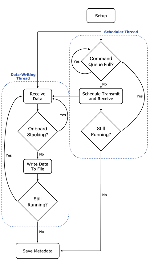
The main radar code is contained in main.cpp (with some SDR setup code located in rf_settings.cpp). The radar code runs in two threads, as shown in the figure below.

One thread is responsible for scheduling timed commands that are enqueued into FIFO queues within the SDR’s FPGA.

The other thead is responsible for pulling received samples from the SDR and writing them to a file on the host computer.

For a more complete overview, please refer to our paper:

T. O. Teisberg, A. L. Broome and D. M. Schroeder, “Open Radar Code Architecture (ORCA): A Platform for Software-Defined Coherent Chirped Radar Systems,” in IEEE Transactions on Geoscience and Remote Sensing, vol. 62, pp. 1-11, 2024, Art no. 5109411, doi: 10.1109/TGRS.2024.3446368.

1.3 - Radar Code

1.3.1 - Configuration options

The entire configuration that controls the radar is defined in a single configuration file. This file is provided at runtime to run.py and encapsulates all of the settings needed to run various experiments on different hardware setups. Configuration files are specified in the YAML format and contained in the config/ folder of the ORCA repository. Default configuration files are included to run the code on a B205mini-i (default_b205.yaml1) and on an X310 (default_x310.yaml). Here we explain the basics behind the settings available to the user via the config file.

Chirp and Pulse Parameters

• sample_rate: Sample rate of the generated chirp (used as TX and RX rate too), specified in Hz
  • On the X310, the sample rate should be an even integer division of the main clock rate
• chirp_type: Chirp frequency progression type
  • Supported options: “linear”, “hyperbolic”
• chirp_bandwidth: Bandwidth of the chirp, specified in Hz
  • Should be less than or equal to sample_rate to satisfy Nyquist
• lo_offset_sw: Center frequency of the chirp, relative to RF0:freq (the RF center frequency), specified in Hz
• window: Window function applied to the chirp
  • Supported options: “rectangular”, “hamming”, “blackman”, “kaiser10”, “kaiser14”, “kaiser18”
  • Applied on transmit and receive by default
• chirp_length: Chirp length without zero padding, specified in seconds
• pulse_length: Total pulse length (chirp + symmetric zero padding), specified in seconds
  • set equal to chirp_length if no zero padding is desired
• out_file: Name of the output binary file containing pulse samples
• show_plot: Whether to display a time-domain plot of the generated chirp (True or False)

Device Connection and Data Transfer Parameters

• device_args: USRP device arguments are used to identify specific SDRs (if multiple areconnected to the same computer), to configure model-specific parameters, and to set transport parameters of the link (USB, ethernet) between the SDR and the host computer.
  • See the default config file or Ettus UHD examples for the SDR you wish to use to set appropriately
• subdev: Active SDR submodules
  • See the default config file or Ettus UHD examples for the SDR you wish to use to set appropriately
• clk_ref: SDR clock reference source
  • Supported options: “internal”, “external”, “gpsdo”
  • “external” requires an external clock reference connected to the SDR
  • “gpsdo” requires a GPSDO module to be installed on the SDR
• clk_rate: SDR main clock frequency, specified in Hz
  • only specific frequencies are allowable for each SDR, see Ettus documentation for more information
• tx_channels: list of TX channels to use (comma separated)
• rx_channels: list of RX channels to use (comma separated)
• cpu_format: CPU-side sample format
  • Supported options: “fc32”, “sc16”, “sc8”
• otw_format: On the wire format
  • any format supported

GPIO Configuration Parameters

Many of the Ettus SDRs have GPIO pins which can be used for conveying automatic transmit/receive signals or other general signals to external devices. The parameters in this section are specific to how MAPPERR and PEREGRINE use the SDR GPIO and can be adapted for other use cases.

• gpio_bank: Which GPIO bank to use
  • “FP0” is the front panel and default bank on the X310
• pwr_amp_pin: Which GPIO pin to use fo external power amplifier control
  • set to “-1” if not using
• ref_out: Turns the 10 MHz reference out signal on the X310 on (1) or off (0)
  • set to (-1) if the SDR does not support a 10 MHz reference out signal

RF Frontend 0 Configuration Parameters

RF configuration parameters for a single-channel radar setup.

• rx_rate: RX sample rate, specified in Hz
  • defaults to be equal to sample_rate
• tx_rate: TX sample rate, specified in Hz
  • defaults to be equal to sample_rate
• freq: Center frequency (LO/mixer frequency), specified in Hz
• lo_offset: hardware LO/mixer offset, specified in Hz
• rx_gain: RX gain, specified in dB
  • available gain range dependent on specific SDR
• tx_gain: TX gain, specified in dB
  • available gain range dependent on specific SDR
• bw: Configurable hardware filter bandwidth, specified in Hz
  • not supported on all SDRs
  • set to 0 if not supported
• tx_ant: Port to be used for TX
• rx_ant: Port to be used for RX
• transmit: Whether to transmit data samples or not
  • set to “true” (or leave blank) to transmit samples (normal operation)
  • set to “false” to completely disable transmit
• tuning_args: Set integer-N or fractional tuning arguments
  • only supported on some SDRs
  • leave as "" to do nothing

RF Frontend 1 Configuration Parameters

RF configuration parameters for the second channel of a multi-channel radar setup. This is only supported on SDRs with more than 2 TX/RX ports. Parameters are the same as in RF Frontend 0 Configuration.

Pulse Timing Parameters

• time_offset: Offset time after set up before the first received sample, specified in seconds
• tx_duration: Transmission duration, specified in seconds
  • defaults as, and should be, equal to pulse_length
• rx_duration: Receive duration, specified in seconds
  • should be long enough to capture echoes from the expected most distant target
• pulse_rep_int: pulse repetition interval, specified in seconds
  • should be longer than or equal to rx_duration
• error_recovery_time: Additional time added (on top of pulse_rep_int) to the next scheduled set of commands after an error occurs.
  • Most errors are due to a command being enqueued too late, so providing some extra buffer time lets the host computer “catch up”
• tx_lead: Time between start of TX and RX, specified in seconds
  • can be used for psuedo-blanking
• num_pulses: Number of chirps/pulses to transmit and receive
  • set to -1 to continuously transmit and record until stopped by CTRL-C
  • code will record num_pulses of error-free pulses before terminating
• num_presums: Number of received pulses to coherently average before writing to file
• phase_dithering: Whether to enable phase dithering or not

During Recording File Location Parameters

• chirp_loc: Which chirp file to transmit
  • in most cases, should be the same as out_file
• save_loc: (Temporary) location to write received samples to
• gps_loc: (Temporary) location to save GPS data
  • only works if “gpsdo” is selected for clk_ref
• max_chirps_per_file: Maximum number of chirps (after presumming) to write to a single file
  • set to -1 to avoid breaking into multiple files

File Save Locations for run.py

These settings are only used by run.py, they are not read by main.cpp.

• final_save_loc: Save location for the big final file, set to null if you don’t want to save a big file
  • if max_chirps_per_file -= -1 (i.e. all data will be written directly to a single file), then final_save_loc and save_partial_files will be ignored
• save_partial_files: Set to True if you want individual small files to be copied with the timestamp, set to False if you just want the big merged file to be copied with the timestamp
  • if max_chirps_per_file == -1 (i.e. all data will be written directly to a single file), then final_save_loc and save_partial_files will be ignored
• save_gps: Set to True if using GPS and wanting to save GPS location data, set to False otherwise

1.3.2 - Host computer transport parameter tuning

The maximum duty cycle you can achieve is a function of the SDR you use, the host computer, and the bandwidth you need. This page outlines suggestions for how to figure out an achievable duty cycle and what parameters can be tweaked to maximize this.

General process for benchmarking duty cycle

Determine the maximum achievable bandwidth with benchmark_rate

Use the USRP example benchmark_rate program (located at <path to conda install>/envs/<uhd environment name>/lib/uhd/examples) to determine the approximate maximum duty cycle you can achieve. For instance, with a Pi 4 and b205mini, I can reach about a 25% duty cycle – defined as sample rate divided by desired sample rate (14 Msps / 56 Msps in this case) – while consistently getting 0 dropped packets.

./benchmark_rate --tx_rate 14e6 --rx_rate 14e6 --tx_otw sc12 --rx_otw sc12 --args="num_recv_frames=512,num_send_frames=512,recv_frame_size=16000,send_frame_size=16000"

This is also the stage to experiment with what transport parameters allow for the highest throughput on your combination of computer/interface/SDR. However the choice of (send/recv)_frame_size should be based on the number of samples per chirp and won’t have the same kind of impact in this continuous streaming case. In other words, you can get close but more tweaking later will help – probably.

Read about USB transport parameters on the Ettus website.

Figure out desired pulse lengths (RX and TX) and set frame sizes appropriately

Basically you want one full set of received samples to fit in a frame. See many more details about this in “Transport layer - throughput limitations” below.

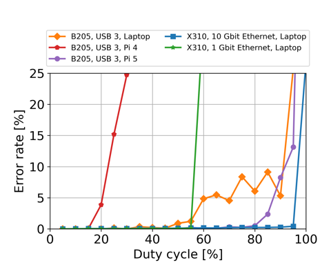
Run tests/error_code_late_command_sweep.py to figure out your max duty cycle

This will sweep across effective duty cycles from 100% to 1, testing the equivalent pulse_rep_int for each one. The script produces a plot (saved as error_code_late_command.png) that shows percent of errors versus duty cycle.

Tuning transport parameters

In addition to getting late commands, the other issues we can run into are overflows (D on network-based devices, O on other devices) and underflows (U on all devices). There are also sequence errors (S) that often go along with late commands (L). Overflows mean that the buffers filled up and samples from the SDR are not being consumed fast enough. Underflows mean that the SDR did not receive samples to transmit before it needed to transmit those samples.

The Ettus knowledge base has a page detailing theoretical maximum transfer rates for each device.

Depending on the device, data is transferred over USB using libUSB, GigE, 10GigE, or PCI-E. For each option, there are various tunable parameters that impact the packet sizes and buffers used.

For libUSB, the transport parameters are:

(send/recv)_frame_size is the maximum packet payload size in bytes. The maximum number of samples that fits into a packet is <packet size in bytes>/<bytes per sample>. The bytes per sample is determined by the over-the-wire format (see otw_format). For example, sc12 requires 24 bit/samples, which is 3 bytes. It’s named sc12 because each value is 12 bits, but there are two values per samples (I, Q).

You can query the max number of samples based on your selected (send/recv)_frame_size through the TX or RX streamers: tx_stream->get_max_num_samps() or rx_stream->get_max_num_samps()

The default is around 8 MB (on my laptop and on the Pi 4B, both running Ubuntu-derived variants). If you set it too high, you’ll get an error message.

In most cases one full chirp (TX) or the received samples associated with one full chirp should fit and a good choice is to set the frame sizes to be equal to (or just barely larger than) the expected number of TX and RX samples, respectively, per chirp.

num_(send/recv)_frames controls how many buffers of size (send/recv)_frame_size are created. The more buffers you allocate for receiving, the longer your host program can lag for before causing an overflow.

LibUSB will give you a memory error if you try to allocate too much memory overall (roughly frame size * number of frames).

This is also why you don’t want arbitrarily large frame sizes. You end up wasting RAM if you’re allocating buffers that are longer than the maximum packet size you expect.

num_recv_frames is one of the most commonly talked about points on the USRP mailing list for throughput issues on the b2xx devices. Apparently the default value is very small (though I wasn’t able to figure out how to find the actual default).

You set these parameters in the device arguments string. For us, that means something like this in the config YAML:

device_args: "num_recv_frames=700,num_send_frames=700,recv_frame_size=11000,send_frame_size=11000"

As described above, the USRP example program benchmark_rate is very useful for playing with these parameters quickly and figuring out what the limits are.

The host side matters a lot here too. The amount of RAM available on the host directly limits the num_(send/recv)_frames. Processing speed of the host in general can easily be the bottleneck. Finally, some USB 3.0 controllers are known to work better than others. The Ettus knowledge base used to have a table of performance on a few selected USB controllers. An archive of that page is available here.

(The Pi 4 uses a VL805 controller. The Pi 5 has a new USB controller that performs far better.)

1.4 - Hardware Setup

In order to standardize between units, much of the Pi setup is automated or semi-automated. This guide will walk you through the steps of setting up your Pi the way we do. Along the way, there are also links for more information on how to customize this setup. This is an area where you will almost certainly need to customize some aspects of the setup.

Initial setup with cloud-init

Setup of the Raspberry Pi is semi-automated using cloud-init.

Cloud-init customization

The cloud-init setup is controlled by two files: user-data and network-config. (You’ll use these files a couple of steps down.)

Examples of each are shown below, but you will likely need to modify these to suit your purpose. We have pages on how to customize user-data and network-config.

user-data Example

#cloud-config

# This is the user-data configuration file for cloud-init.
# The cloud-init documentation has more details:
#
# https://cloudinit.readthedocs.io/

system_info:
  default_user:
    name: ubuntu # Allow the default user to shutdown or reboot the system without entering a password (used by our automated scripts)
    sudo: "ALL=(ALL) NOPASSWD: /sbin/poweroff, /sbin/reboot, /sbin/shutdown"

# On first boot, set the (default) ubuntu user's password to "cryosphere"
chpasswd:
  expire: false
  users:
    - name: ubuntu
      password: $6$rounds=4096$aQ7tu0.beL3WAL32$fKxKYvZpY7EMCoxAU1heRomA3v8WvgbqBhhz08QwOtQdlP/DJOP2BThqZFoRW8d2a9PaIKK9BC9NHs1qNnkya1
      type: hash

# Enable password authentication with the SSH daemon
ssh_pwauth: true

# Set a default timezone
timezone: Etc/UTC

## Update apt database and upgrade packages on first boot
package_update: true
package_upgrade: true

## Install additional packages on first boot
packages:
- net-tools
- git
- cmake
- g++
- mosh
- exfat-fuse
- i2c-tools
- rpi.gpio-common
- util-linux-extra
- gpsd
- gpsd-clients

## Write arbitrary files to the file-system
write_files:
- path: /home/ubuntu/initial_setup.sh
  content: |
    #!/bin/bash
    exec > >(tee -a "initial_setup_output.log") 2>&1
    # Miniconda Setup
    wget --progress=bar:force:noscroll "https://github.com/conda-forge/miniforge/releases/latest/download/Miniforge3-Linux-aarch64.sh" -O $HOME/miniconda.sh
    bash $HOME/miniconda.sh -b -p $HOME/miniconda
    cd $HOME
    source .profile
    source miniconda/etc/profile.d/conda.sh
    conda init bash
    # Setup logger environment
    git clone git@github.com:thomasteisberg/uav_radar_logger.git
    # Clone uhd_radar repo
    git clone git@github.com:radioglaciology/uhd_radar.git
    cd uhd_radar
    #git checkout thomas/dask # Uncomment if you want to check out a specific branch other than main
    conda env create -n uhd -f environment-rpi.yaml
    conda activate uhd
    python /home/ubuntu/miniconda/envs/uhd/lib/uhd/utils/uhd_images_downloader.py
    systemctl --user enable radar.service
    systemctl --user enable logger.service
    ifconfig
    sudo reboot
  append: true
- path: /home/ubuntu/.profile
  content: |
    PATH=/home/ubuntu/miniconda/bin:$PATH
    source /home/ubuntu/.bashrc
  append: true
- path: /home/ubuntu/.ssh/known_hosts
  content: |
    github.com ssh-ed25519 AAAAC3NzaC1lZDI1NTE5AAAAIOMqqnkVzrm0SdG6UOoqKLsabgH5C9okWi0dh2l9GKJl
    github.com ecdsa-sha2-nistp256 AAAAE2VjZHNhLXNoYTItbmlzdHAyNTYAAAAIbmlzdHAyNTYAAABBBEmKSENjQEezOmxkZMy7opKgwFB9nkt5YRrYMjNuG5N87uRgg6CLrbo5wAdT/y6v0mKV0U2w0WZ2YB/++Tpockg=
    github.com ssh-rsa AAAAB3NzaC1yc2EAAAADAQABAAABgQCj7ndNxQowgcQnjshcLrqPEiiphnt+VTTvDP6mHBL9j1aNUkY4Ue1gvwnGLVlOhGeYrnZaMgRK6+PKCUXaDbC7qtbW8gIkhL7aGCsOr/C56SJMy/BCZfxd1nWzAOxSDPgVsmerOBYfNqltV9/hWCqBywINIR+5dIg6JTJ72pcEpEjcYgXkE2YEFXV1JHnsKgbLWNlhScqb2UmyRkQyytRLtL+38TGxkxCflmO+5Z8CSSNY7GidjMIZ7Q4zMjA2n1nGrlTDkzwDCsw+wqFPGQA179cnfGWOWRVruj16z6XyvxvjJwbz0wQZ75XK5tKSb7FNyeIEs4TT4jk+S4dhPeAUC5y+bDYirYgM4GC7uEnztnZyaVWQ7B381AK4Qdrwt51ZqExKbQpTUNn+EjqoTwvqNj4kqx5QUCI0ThS/YkOxJCXmPUWZbhjpCg56i+2aB6CmK2JGhn57K5mj0MNdBXA4/WnwH6XoPWJzK5Nyu2zB3nAZp+S5hpQs+p1vN1/wsjk=
- path: /etc/security/limits.conf # Recommended by Ettus https://kb.ettus.com/USRP_Host_Performance_Tuning_Tips_and_Tricks
  content: |
    ubuntu    - rtprio    99
  append: true
- path: /etc/systemd/user/radar.service
  content: |
    [Unit]
    Description=Service to run the radar code on startup

    [Service]
    Type=simple
    WorkingDirectory=/home/ubuntu/uhd_radar/
    ExecStart=/home/ubuntu/uhd_radar/manager/radar_service.sh

    Restart=always
    RestartSec=10

    KillSignal=SIGINT

    [Install]
    WantedBy=default.target
- path: /etc/systemd/user/logger.service
  content: |
    [Unit]
    Description=Service to log data from I2C sensors and automatically shutdown below a voltage threshold

    [Service]
    Type=simple
    WorkingDirectory=/home/ubuntu/uav_radar_logger/
    ExecStart=/home/ubuntu/uav_radar_logger/logger_service.sh

    Restart=always
    RestartSec=60

    KillSignal=SIGINT

    [Install]
    WantedBy=default.target

# Run arbitrary commands at rc.local like time
# These commands are run with root permissions
# If you want commands run as a normal user, put them in initial_setup.sh (see above)
# which is run as the "ubuntu" user (see below)
runcmd:
- chown -R ubuntu:ubuntu /home/ubuntu
- chmod +x /home/ubuntu/initial_setup.sh
- wget -O /etc/udev/rules.d/uhd-usrp.rules https://raw.githubusercontent.com/EttusResearch/uhd/master/host/utils/uhd-usrp.rules
- usermod -a -G i2c ubuntu
- usermod -a -G dialout ubuntu
- usermod -a -G tty ubuntu
- apt remove -y modemmanager
- systemctl stop serial-getty@ttyS0.service && systemctl disable serial-getty@ttyS0.service
- i2cdetect -y 1
- echo "dtoverlay=i2c-rtc,pcf8523" >> /boot/firmware/config.txt
- loginctl enable-linger ubuntu
- mkdir /media/ssd
- chown ubuntu /media/ssd
- chgrp ubuntu /media/ssd
- echo "/dev/sda2  /media/ssd  exfat  defaults,nofail,uid=1000,gid=1000  0  2" | tee -a /etc/fstab

network-config Example

# This file contains a netplan-compatible configuration which cloud-init will
# apply on first-boot (note: it will *not* update the config after the first
# boot). Please refer to the cloud-init documentation and the netplan reference
# for full details:
#
# https://cloudinit.readthedocs.io/en/latest/topics/network-config.html
# https://cloudinit.readthedocs.io/en/latest/topics/network-config-format-v2.html
# https://netplan.io/reference

version: 2
ethernets:
  eth0:  # Your ethernet name.
    dhcp4: no
    addresses: [192.168.11.137/24]
    gateway4: 192.168.11.1
    nameservers:
      addresses: [8.8.8.8,8.8.4.4]
wifis:
  renderer: networkd
  wlan0:
    dhcp4: true
    optional: true
    access-points:
      "<YOUR WIFI SSID HERE>":
        password: "<YOUR WIFI PASSWORD HERE>"

Imaging your Pi

To start, download the Raspberry Pi Imager tool (or use your preferred software for imaging SD cards). On Ubuntu, you can install it like this:

sudo apt install rpi-imager

For other operating systems, see the website.

Launch Imager. After clicking on “Choose OS,” navigate through the general purpose category to find Ubuntu Server 22.04.xx LTS 64-bit. 64-bit is important – 32-bit will not work.

Insert your MicroSD card and select it as the location to write to.

After imaging is complete, you will see two drives mounted: writable and system-boot.

Copying cloud-init config files

After customizing the user-data and network-config files (see above), copy user-data and network-config to the system-boot volume, replacing the existing files.

Eject the microSD and put it back in the Pi.

Running cloud-init

Power up the Pi and wait for cloud-init to run.

Within about a minute, your Pi should connect to whatever network interface(s) are described in network-config and you should be able to find it on the network. If you setup some sort of key-based authentication (such as by importing a key from GitHub), it may take an extra couple of minutes for this to be ready.

After the network setup is complete, you should be able to login over SSH.

In particular, please note that you need to have SSH agent forwarding working. Instructions for this are on that page.

When you first login, cloud-init may not have finished running. To check the status, run:

cloud-init status --long

There are also logs in /var/log/cloud-init-output.log.

To keep an eye on the entire process, you can run:

watch "cloud-init status --long && tail -n 10 /var/log/cloud-init-output.log"

Expect this process to take a few minutes to complete.

Running initial_setup.sh

After the cloud-init process is complete, you’ll also need to run initial_setup.sh:

./initial_setup.sh

This will log to /home/ubuntu/initial_setup_output.log. It may take around 10 minutes to complete. It will automatically reboot your Pi at the end. If you don’t want this, feel free to comment out the last line.

Setting up the logger service

More details on the logging service will eventually be here.

For now, if you’re building a Peregrine system, the default setup should be fine.

If you’re building Eyas, first run this command to create a place for logs:

mkdir /media/ssd/logger

And then modify the last line of /home/ubuntu/uav_radar_logger/logger_service.sh to look like this:

python -u logger.py --shutdown-voltage 11.8 --log-dir /media/ssd/logger/

Replacing 11.8 with an appropriate threshold (in volts) at which to shutdown.

Setting up the radar service

More details on the radar service will eventually be here.

For now, if you’re building a Peregrine system, the default setup should be fine.

If you’re building Eyas, run these commands to create a location for logging data and update the default configuration:

mkdir /media/ssd/radar
cd /home/ubuntu/uhd_radar/config
mv default.yaml default-old.yaml
cp default-eyas.yaml default.yaml

Using overlayroot to protect the file system

Let’s take a quick step back and talk about the problem before we talk about (perhaps drastic) solutions:

MicroSD card corruption is an ongoing challenge for any device (such as the Pi) that boots from a MicroSD card. Most cases can be traced to either (a) junk MicroSD cards or (b) sudden power loss during a write operation.

You can mostly avoid problem (a) by carefully sourcing your MicroSD cards. If you’re considering saving $20 by buying an off-brand MicroSD card or, worse, a possible fake, don’t do it.

Sudden power loss is harder to completely guard against. Ideally, you want to shutdown your Pi before removing power. This can be done by SSH-ing into it and running sudo shutdown -h now and waiting about a minute. If you use our radar systemd service, you can also perform a safe shutdown by pressing and holding the button for 5 seconds, waiting for the light to turn off, and then giving it about a minute to fully shut down.

For Peregrine, this should all be good enough.

For Eyas and other longer-term installations, the risk of a battery discharging faster than expected is relatively high.

The first line of defense is the automatic shutdown provided by the logger service that will safely shut everything down when the battery voltage gets too low.

If you have a separate data storage device, such as an external USB-connected SSD, you can go a step further and make your Pi’s MicroSD card read-only.

A utility called overlayroot (which uses OverlayFS) can be used to make the root filesystem read-only and create an “overlay filesystem” stored only in RAM. This means that all changes to the MicroSD card file system are temporary and are lost upon reboot.

This is great for keeping a standardized configuration, but you need to be aware that this means most log files are lost on reboot, any config files on the SD card are lost on reboot, and all radar data you want to keep around must be stored to your external storage device.

You can read a more detailed tutorial about Overlayroot here.

If you’re going to do this, be sure that you’ve tested your setup in advance so you know if the data you want to keep is being stored.

Enabling Overlayroot

If you still want to set this up, it’s quite easy to enable.

Simply edit the last line of /etc/overlayroot.conf to this:

overlayroot="tmpfs:recurse=0"

tmpfs specifies that we want to use a RAM-based filesystem to store the “overlay” part of the filesystem. recurse=0 says that we want to apply this only to the / mount and not to other mounts below that.

(You need to edit this file as root. For example: sudo vim /etc/overlayroot.conf)

Disabling Overlayroot

You can temporarily re-mount the root filesystem to edit things using the built-in utility:

sudo overlayroot-chroot

To exit, just type exit.

If you want to permenantly disable it, just edit the last line of /etc/overlayroot.conf back to:

overlayroot=""

and reboot.

Step-by-step Installation Guide

The following guide is for Windows, however the steps are the same for Linux and MacOS with some minor tweaks (no need to install WSL, filepaths may differ, etc).

Installing Software

1. Install Visual Studio Code (VSCode) or another code editor of your choice.

   If you are using VSCode, see the additional steps for setting it up here.

2. Install Windows Subsystem for Linux (WSL). ORCA is developed to be used on a Linux system and requires a Linux terminal such as WSL to run.

   From the Start menu, open Powershell and run wsl --install.

3. Download Conda for Linux. In this guide, we use Miniconda. More details about Conda can be found here. You do not need to open or run the .sh file at this time.

4. Within VSCode, open a new Ubuntu (WSL) terminal. You may be prompted to create a username and password for the Linux installation. This password will be used any time you run WSL terminal commands with administrator permissions (sudo).

5. In the WSL terminal, run bash <path-to-Downloads>/Miniconda3-latest-Linux_x86_64.sh. The path to your downloads folder is typically /mnt/c/Users/<your-username>/Downloads. Accept the default options when prompted, and select yes when asked about auto_activate_base, though we will change this setting later.

6. After Miniconda has been installed, close and reopen the WSL terminal, then run conda list to confirm everything has been installed correctly. You should see a long list of all the installed dependencies printed to the terminal. If you get an error saying conda: command not found, you may be in the wrong terminal or did not install it correctly.

7. We are now going to disable conda from activating every time you open a new terminal. To do this, run conda config --set auto_activate_base false.

Connecting to GitHub

If you do not intend to modify the code in any way, you may skip this section.

1. Create an account on GitHub and sign in.
2. Go to the ORCA Repository and click Fork to create your own copy of the code. Name this new repository whatever you want.
3. To securely connect your computer to GitHub we will create an SSH key. In the WSL terminal, run ssh-keygen -t ed25519 -C "your@email.com" and accept the default location.
4. Create a password that you will input each time you push or pull code from GitHub. When you type the password, no text will appear in the terminal but the password is being logged.
5. We now need to copy the public key you just created. When the key was generated, a message should have been printed that says something like Your public key has been saved in /home//.ssh/id_ed25519.pub. To view the contents of this public key file, run cat /home/<your-username>/.ssh/id_ed25519.pub and copy the full key that is printed to the terminal.
6. In GitHub. open Settings > SSH and GPG Keys, and click New SSH Key, then paste the key into the appropriate box.

Cloning the Repository

1. We now need to install Git in WSL. Run sudo apt update && sudo apt install git.
2. To be able to access the code from GitHub on your computer, we have to clone the repository. Go to the fork you just created (or the ORCA repository if you are not creating a fork), and click the green Code button. Within the dropdown, go to the SSH tab and copy the link. It should end in .git.
3. Navigate (cd) to whichever folder you would like the code to be copied into, and run git clone <link-to-repo>.
4. In VSCode, you can now view the code with File > Open Folder.

Setting up Conda

1. We now need to use Conda to install the required dependencies for ORCA.
2. Before we create the conda environment, check that GCC is installed by running gcc --version in the WSL terminal. If the gcc command is not found, install it with sudo apt update && sudo apt install gcc.
3. Navigate to the folder containing the code. If you are using a Raspberry Pi to control the SDR, then use environment-rpi.yaml in the next step instead. Run conda env create -f environment.yaml.
4. Once the environment is installed, activate it with conda activate uhd.
5. Finally, we need to install any remaining dependencies for compiling the code, such as make. To install them, run sudo apt update and sudo apt install build-essential.

The code is now installed and ready to be compiled and run, either manually or using the run.py script provided.

1.4.1 - Compatible hardware

Selecting a Software-Defined Radio (SDR)

ORCA is built upon the USRP Hardware Driver (UHD). As such, it is theoretically compatible with any Ettus SDR. We have primarily tested with B and X series devices (B205mini and X310, in particular), however most other Ettus SDRs should work with minor tweaks.

The basic capabilities of the two models we regularly use are detailed below:

In general, we recommend B series devices for applications with constraints on size, weight, power, or budget. When capabilities beyond the B series are needed, we recommend the X series.

If no device in either series suits your needs, consider other Ettus SDRs. Most should work with minor tweaks. The exception to note are E series devices, which include an embedded computer running Linux. In theory, this code could be run on that embedded computer, however the performance limitations would limit the use cases.

Host Computer

Unless you choose an E series device (see caution above), you will also need a computer to interface with the SDR. This computer is where the ORCA code will run.

The capabilities of the computer can make a significant difference in the system performance. The host computer must support an interface with enough bandwidth for the samples you want to transfer and be able to store these samples to an appropriate storage medium.

If you’re not resource constrained, a modern laptop will provide more than enough processing power, as long as it supports the interface you need. Keep in mind that X-series SDRs need a 10 gigabit ethernet (10 GigE) interface to achieve maximum sample rates. Few laptops natively support 10 GigE, however there are Thunderbolt adapters available. (Not all USB C ports support Thunderbolt and it may not be available on low-end laptops.)

For an embedded solution, Raspberry Pi’s are suitable for working with B series devices. The performance of the Raspberry Pi 5 greatly exceeds the Raspberry Pi 4, likely due to the introduction of a new USB interface chip.

Some caution is advised with other single-board computers. Their performance will likely be limited by their choice of USB controller chip.

For some examples of duty cycles achievable with various combinations of SDRs and host computers, see the figure below. Note that actual performance will depend on a variety of factors, including your exact configuration and the speed of your storage medium.

1.4.2 - 2 - Default Setup for the Raspberry Pi

Use this when setting up your Raspberry Pi on initial boot-up.

The default user-data we start from is as shown below. You will likely need to tweak many of these settings. Descriptions and tips for the most important sections are below.

Note that this is one of two key configuration files. You can read about network-config here.

Starting point user-data file

#cloud-config

# This is the user-data configuration file for cloud-init.
# The cloud-init documentation has more details:
#
# https://cloudinit.readthedocs.io/

system_info:
  default_user:
    name: ubuntu # Allow the default user to shutdown or reboot the system without entering a password (used by our automated scripts)
    sudo: "ALL=(ALL) NOPASSWD: /sbin/poweroff, /sbin/reboot, /sbin/shutdown"

# On first boot, set the (default) ubuntu user's password to "cryosphere"
chpasswd:
  expire: false
  users:
    - name: ubuntu
      password: $6$rounds=4096$aQ7tu0.beL3WAL32$fKxKYvZpY7EMCoxAU1heRomA3v8WvgbqBhhz08QwOtQdlP/DJOP2BThqZFoRW8d2a9PaIKK9BC9NHs1qNnkya1
      type: hash

# Enable password authentication with the SSH daemon
ssh_pwauth: true

# Set a default timezone
timezone: Etc/UTC

## Update apt database and upgrade packages on first boot
package_update: true
package_upgrade: true

## Install additional packages on first boot
packages:
- net-tools
- git
- cmake
- g++
- mosh
- exfat-fuse
- i2c-tools
- rpi.gpio-common
- util-linux-extra
- gpsd
- gpsd-clients

## Write arbitrary files to the file-system
write_files:
- path: /home/ubuntu/initial_setup.sh
  content: |
    #!/bin/bash
    exec > >(tee -a "initial_setup_output.log") 2>&1
    # Miniconda Setup
    wget --progress=bar:force:noscroll "https://github.com/conda-forge/miniforge/releases/latest/download/Miniforge3-Linux-aarch64.sh" -O $HOME/miniconda.sh
    bash $HOME/miniconda.sh -b -p $HOME/miniconda
    cd $HOME
    source .profile
    source miniconda/etc/profile.d/conda.sh
    conda init bash
    # Setup logger environment
    git clone git@github.com:thomasteisberg/uav_radar_logger.git
    # Clone uhd_radar repo
    git clone git@github.com:radioglaciology/uhd_radar.git
    cd uhd_radar
    #git checkout thomas/dask # Uncomment if you want to check out a specific branch other than main
    conda env create -n uhd -f environment-rpi.yaml
    conda activate uhd
    python /home/ubuntu/miniconda/envs/uhd/lib/uhd/utils/uhd_images_downloader.py
    systemctl --user enable radar.service
    systemctl --user enable logger.service
    ifconfig
    sudo reboot
  append: true
- path: /home/ubuntu/.profile
  content: |
    PATH=/home/ubuntu/miniconda/bin:$PATH
    source /home/ubuntu/.bashrc
  append: true
- path: /home/ubuntu/.ssh/known_hosts
  content: |
    github.com ssh-ed25519 AAAAC3NzaC1lZDI1NTE5AAAAIOMqqnkVzrm0SdG6UOoqKLsabgH5C9okWi0dh2l9GKJl
    github.com ecdsa-sha2-nistp256 AAAAE2VjZHNhLXNoYTItbmlzdHAyNTYAAAAIbmlzdHAyNTYAAABBBEmKSENjQEezOmxkZMy7opKgwFB9nkt5YRrYMjNuG5N87uRgg6CLrbo5wAdT/y6v0mKV0U2w0WZ2YB/++Tpockg=
    github.com ssh-rsa AAAAB3NzaC1yc2EAAAADAQABAAABgQCj7ndNxQowgcQnjshcLrqPEiiphnt+VTTvDP6mHBL9j1aNUkY4Ue1gvwnGLVlOhGeYrnZaMgRK6+PKCUXaDbC7qtbW8gIkhL7aGCsOr/C56SJMy/BCZfxd1nWzAOxSDPgVsmerOBYfNqltV9/hWCqBywINIR+5dIg6JTJ72pcEpEjcYgXkE2YEFXV1JHnsKgbLWNlhScqb2UmyRkQyytRLtL+38TGxkxCflmO+5Z8CSSNY7GidjMIZ7Q4zMjA2n1nGrlTDkzwDCsw+wqFPGQA179cnfGWOWRVruj16z6XyvxvjJwbz0wQZ75XK5tKSb7FNyeIEs4TT4jk+S4dhPeAUC5y+bDYirYgM4GC7uEnztnZyaVWQ7B381AK4Qdrwt51ZqExKbQpTUNn+EjqoTwvqNj4kqx5QUCI0ThS/YkOxJCXmPUWZbhjpCg56i+2aB6CmK2JGhn57K5mj0MNdBXA4/WnwH6XoPWJzK5Nyu2zB3nAZp+S5hpQs+p1vN1/wsjk=
- path: /etc/security/limits.conf # Recommended by Ettus https://kb.ettus.com/USRP_Host_Performance_Tuning_Tips_and_Tricks
  content: |
    ubuntu    - rtprio    99
  append: true
- path: /etc/systemd/user/radar.service
  content: |
    [Unit]
    Description=Service to run the radar code on startup

    [Service]
    Type=simple
    WorkingDirectory=/home/ubuntu/uhd_radar/
    ExecStart=/home/ubuntu/uhd_radar/manager/radar_service.sh

    Restart=always
    RestartSec=10

    KillSignal=SIGINT

    [Install]
    WantedBy=default.target
- path: /etc/systemd/user/logger.service
  content: |
    [Unit]
    Description=Service to log data from I2C sensors and automatically shutdown below a voltage threshold

    [Service]
    Type=simple
    WorkingDirectory=/home/ubuntu/uav_radar_logger/
    ExecStart=/home/ubuntu/uav_radar_logger/logger_service.sh

    Restart=always
    RestartSec=60

    KillSignal=SIGINT

    [Install]
    WantedBy=default.target

# Run arbitrary commands at rc.local like time
# These commands are run with root permissions
# If you want commands run as a normal user, put them in initial_setup.sh (see above)
# which is run as the "ubuntu" user (see below)
runcmd:
- chown -R ubuntu:ubuntu /home/ubuntu
- chmod +x /home/ubuntu/initial_setup.sh
- wget -O /etc/udev/rules.d/uhd-usrp.rules https://raw.githubusercontent.com/EttusResearch/uhd/master/host/utils/uhd-usrp.rules
- usermod -a -G i2c ubuntu
- usermod -a -G dialout ubuntu
- usermod -a -G tty ubuntu
- apt remove -y modemmanager
- systemctl stop serial-getty@ttyS0.service && systemctl disable serial-getty@ttyS0.service
- i2cdetect -y 1
- echo "dtoverlay=i2c-rtc,pcf8523" >> /boot/firmware/config.txt
- loginctl enable-linger ubuntu
- mkdir /media/ssd
- chown ubuntu /media/ssd
- chgrp ubuntu /media/ssd
- echo "/dev/sda2  /media/ssd  exfat  defaults,nofail,uid=1000,gid=1000  0  2" | tee -a /etc/fstab

Password-less shutdown

system_info:
  default_user:
    name: ubuntu # Allow the default user to shutdown or reboot the system without entering a password (used by our automated scripts)
    sudo: "ALL=(ALL) NOPASSWD: /sbin/poweroff, /sbin/reboot, /sbin/shutdown"

One of the features supported by the uav_radar_logger utility is to automatically cleanly shutdown the system if the measured battery voltage drops below a threshold. To facilitate this, the default user must be able to shutdown the system without needing additional authentication. This gives permission for the ubuntu user to call sudo shutdown or sudo reboot without entering a password.

Password authentication

# On first boot, set the (default) ubuntu user's password to "cryosphere"
chpasswd:
  expire: false
  list:
  - ubuntu:$6$rounds=4096$aQ7tu0.beL3WAL32$fKxKYvZpY7EMCoxAU1heRomA3v8WvgbqBhhz08QwOtQdlP/DJOP2BThqZFoRW8d2a9PaIKK9BC9NHs1qNnkya1

# Enable password authentication with the SSH daemon
ssh_pwauth: true

This sets up a default password for the ubuntu user. You should change this to something else (or disable password authentication completely, if you prefer).

Passwords are stored in a hashed format. You can generate password hashes using this utility:

mkpasswd --method=SHA-512 --rounds=4096

Timezone

# Set a default timezone
timezone: Etc/UTC

You could set this to other time zones (i.e. `America/Los_Angeles"), but really it would make everyone’s life easier if you just set your clock to UTC.

Add SSH keys through GitHub

## On first boot, use ssh-import-id to give the specific users SSH access to
## the default user
ssh_import_id:
- gh:thomasteisberg
- gh:albroome
- gh:dfxmay

You can very conveniently enable key-based authentication for specific GitHub user names. If your username is in here and you have a public key setup with GitHub, this public key will be imported and you will be able to SSH into your Pi with no additional setup. You might want to remove us from your list, though. :)

Files

Arbitrary files can be written to the system with cloud-init. Some of these are important.

initial_setup.sh

- path: /home/ubuntu/initial_setup.sh
  content: |
    #!/bin/bash
    exec > >(tee -a "initial_setup_output.log") 2>&1
    # Miniconda Setup
    wget --progress=bar:force:noscroll "https://github.com/conda-forge/miniforge/releases/latest/download/Miniforge3-Linux-aarch64.sh" -O $HOME/miniconda.sh
    bash $HOME/miniconda.sh -b -p $HOME/miniconda
    cd $HOME
    source .profile
    source miniconda/etc/profile.d/conda.sh
    conda init bash
    # Setup logger environment
    git clone git@github.com:thomasteisberg/uav_radar_logger.git
    # Clone uhd_radar repo
    git clone git@github.com:radioglaciology/uhd_radar.git
    cd uhd_radar
    #git checkout thomas/dask # Uncomment if you want to check out a specific branch other than main
    conda env create -n uhd -f environment.yaml
    conda activate uhd
    python /home/ubuntu/miniconda/envs/uhd/lib/uhd/utils/uhd_images_downloader.py
    systemctl --user enable radar.service
    systemctl --user enable logger.service
    ifconfig
    sudo reboot
  append: true

The initial_setup.sh script grabs copies of our code and sets up the radar and logging services. This script is intended to be manually run the first time you SSH into the system. This enables you to use SSH agent forwarding to provide any needed GitHub authentication to get the code.

This is also where you would customize the repositories to check out (if, for example, you’ve forked our code) and where you can pick a branch to automatically checkout.

Radar and Logger services

- path: /etc/systemd/user/radar.service
  content: |
    [Unit]
    Description=Service to run the radar code on startup

    [Service]
    Type=simple
    WorkingDirectory=/home/ubuntu/uhd_radar/
    ExecStart=/home/ubuntu/uhd_radar/manager/radar_service.sh

    Restart=always
    RestartSec=10

    KillSignal=SIGINT

    [Install]
    WantedBy=default.target
- path: /etc/systemd/user/logger.service
  content: |
    [Unit]
    Description=Service to log data from I2C sensors and automatically shutdown below a voltage threshold

    [Service]
    Type=simple
    WorkingDirectory=/home/ubuntu/uav_radar_logger/
    ExecStart=/home/ubuntu/uav_radar_logger/logger_service.sh

    Restart=always
    RestartSec=60

    KillSignal=SIGINT

    [Install]
    WantedBy=default.target

Two systemd services are used to manage everything. One run the radar code in its default button-controlled setup. The other runs basic logging of I2C-connected sensors and handles automatic low-battery shutdown.

Run commands

runcmd:
- chown -R ubuntu:ubuntu /home/ubuntu
- chmod +x /home/ubuntu/initial_setup.sh
- wget -O /etc/udev/rules.d/uhd-usrp.rules https://raw.githubusercontent.com/EttusResearch/uhd/master/host/utils/uhd-usrp.rules
- usermod -a -G i2c ubuntu
- usermod -a -G dialout ubuntu
- usermod -a -G tty ubuntu
- apt remove -y modemmanager
- systemctl stop serial-getty@ttyS0.service && systemctl disable serial-getty@ttyS0.service
- i2cdetect -y 1
- echo "dtoverlay=i2c-rtc,pcf8523" >> /boot/firmware/config.txt
- loginctl enable-linger ubuntu
- mkdir /media/ssd
- echo "/dev/sda2  /media/ssd  exfat  defaults,nofail,uid=1000,gid=1000  0  2" | tee -a /etc/fstab

Some final setup is done by running arbitrary commands. These are run as the root user.

One aspect of this you may wish to customize are the last two lines, which add settings to automatically mount an ExFAT-formatted SSD plugged into the Pi. This can be (optionally) used as a storage location for radar data.

Testing changes

You may want to test your changes before using them on your Pi. Options for doing that are described here. Note that the initial_setup.sh script downloads miniconda for the aarch64 architecture, which probably won’t work on your computer. If you want to test that part, you’ll need to change this.

1.4.3 - Runtime overview

Conda environment setup

All of the required dependencies can be installed as a conda environment using the environment.yaml file in the repository. More instructions can be found in the README file.

Startup scripts

The X series devices require some initial network configuration. For convenience, a startup script is provided to automate this setup. You may need to tweak this file to your setup.

Runner scripts

The basic steps required to run the radar are:

1. Build the C++ code
2. Generate a chirp file to transmit based on your configuration
3. Run the compiled radar code
4. Move the collected data to an appropriate location

The main interface for running the radar code is through run.py, a Python script designed to automate the above process. This script is run as follows:

python run.py config/my_radar_configuration.yaml

At the end of the data collection, data will be saved with the current date to a location specified in the YAML config file.

Generally, three files are saved:

• YYYYMMDD_hhmmss_rx_samps.bin - This is a binary file containing the raw samples recorded the SDR. Note that this file is not interpretable unless you also have the config file used.
• YYYYMMDD_hhmmss_config.yaml - This is the YAML config file passed to run.py. It defines all parameters of the data collection, allowing for the rx_samps.bin file to be interpreted and processed.
• YYYYMMDD_hhmmss_uhd_stdout.log - This is a text file containing the output of running the radar code. This is helpful for debugging and also contains a log of any errors encountered, which may be required to reconstruct the timing of each recording.

More details on the files stored and how these can be re-processed into a Zarr file are on the file formats page.

Note that there are also settings available to break rx_samps.bin into multiple files as needed.

SDR interface code

For performance reasons, the code directly interfacing with the SDR is written in C++. This code is all located in the sdr/ directory of the repository.

The main radar code is contained in main.cpp (with some SDR setup code located in rf_settings.cpp). The radar code runs in two threads, as shown in the figure below.

One thread is responsible for scheduling timed commands that are enqueued into FIFO queues within the SDR’s FPGA.

The other thead is responsible for pulling received samples from the SDR and writing them to a file on the host computer.

For a more complete overview, please refer to our paper:

T. O. Teisberg, A. L. Broome and D. M. Schroeder, “Open Radar Code Architecture (ORCA): A Platform for Software-Defined Coherent Chirped Radar Systems,” in IEEE Transactions on Geoscience and Remote Sensing, vol. 62, pp. 1-11, 2024, Art no. 5109411, doi: 10.1109/TGRS.2024.3446368.

1.4.4 - Connect and Control Options

Most of the time, the Pi doesn’t need an internet connection. There are, however, a couple of cases where you may want some sort of a network connection to the Pi.

These are:

1. Downloading data from the Pi to a computer (requires a network connection but not internet)
2. Initial setup with cloud-init (requires internet)
3. Updating code by pulling from GitHub (requires internet)

There are three potential ways to communicate with the Raspberry Pi; direct control, ethernet, or via Wi-Fi. The Raspberry Pi as set up does not have a graphical user interface (GUI). After initial set-up, if the user wants to add remote access or move files onto the Pi, they wil need to do so using direct control. Direct control uses Secure Shell (ssh) protocol.

Direct Control

To access the Pi’s terminal directly you will need:

1. Raspberry Pi 5
2. Pi Power Supply (plugged into wall)
3. Monitor (plugged into wall)
4. HDMI to Micro-HDMI cable
5. Keyboard
6. Ethernet cable connected to a router (or ethernet port on the wall of the lab)

Connect the ethernet (or just use Wi-Fi), micro-HDMI, keyboard, and power supply to the Raspberry Pi. When it boots, you will see the Pi’s Ubuntu Server terminal on the monitor and can log in and run commands directly with the keyboard (no mouse inputs). There is no way to scroll up through this terminal, so if you want to be able to read a long output from a command you must pipe it into a file (ex. python run.py >> terminal_output.txt), then read the text file using nano.

After you have connected to the Raspberry Pi using direct control, it is possible to configure the computer to use SSH so that you can log in to the Pi on your computer (via Ethernet or via Wi-Fi).

To do so, you need to set up SSH agent forwarding, or confirm that it is already running.

Confirm that SSH agent forwarding (i.e. a remote server can access the local SSH agent on your behalf) is working properly by running ssh -T git@github.com.

SSH Agent Forwarding

If you need to authenticate to GitHub to download code, the recommended way is using SSH agent forwarding.

To summarize the above link, you should make sure you have an SSH key setup with your GitHub account.

Test this by running ssh -T git@github.com.

You should now have permission to SSH into the Pi from your laptop using direct control, ethernet, or Wi-Fi.

Modify your ~/.ssh/config file (use nano ~/.ssh/config) and add an entry like this enabling SSH agent forwarding:

Host 192.168.11.137
    HostName 192.168.11.137
    User ubuntu
    ForwardAgent yes

Note that if your username or host IP address is different, you should adjust it accordingly.

@@@@@@@@@@@@@@@@@@@@@@@@@@@@@@@@@@@@@@@@@@@@@@@@@@@@@@@@@@@
@    WARNING: REMOTE HOST IDENTIFICATION HAS CHANGED!     @
@@@@@@@@@@@@@@@@@@@@@@@@@@@@@@@@@@@@@@@@@@@@@@@@@@@@@@@@@@@
IT IS POSSIBLE THAT SOMEONE IS DOING SOMETHING NASTY!
Someone could be eavesdropping on you right now (man-in-the-middle attack)!
It is also possible that a host key has just been changed.

ssh-keyscan -H 192.168.11.137 >> ~/.ssh/known_hosts

Once this is set up properly, it is possible to connect to the Raspberry Pi through your computer (Ethernet) or through Wi-Fi, so long as the Raspberry Pi remains powered.

SSH over Ethernet

This is the preferred method for connecting to and controlling the Pi, and the only method that does not require the Pi to be connected to a router or Wi-Fi network. However, it does take a bit of setup the first time.

For this method, you will need:

1. Laptop connected to Wi-Fi
2. Raspberry Pi 5
3. Pi Power Supply (plugged into wall)
4. Ethernet cable
5. Ethernet to usb-c adapter (if your laptop doesn’t have an ethernet port)

Configuring your computer

If you’re connecting to the Pi via a simple ethernet cable to your computer, you’ll want both configured with static IPs. The config file above will do this on the Pi side. On your computer, you’ll want to set a static IP of 192.168.11.1 and a netmask of 255.255.255.0. For example, your settings may look like this:

Sharing internet from your computer

Sharing your computer’s internet connection from one network interface to another is a useful trick to get an internet connection for the Pi. This can be done between any two network interfaces (i.e. from your Wi-Fi connection to the Pi over ethernet or from one WiFi card to a network created by a second Wi-Fi card).

The Arch Linux wiki has useful instructions for configuring internet sharing on Linux.

To briefly summarize them:

All of this setup will happen on your laptop (or whatever computer has an internet connection).

1. Enable IPv4 forwarding: sudo sysctl net.ipv4.ip_forward=1
2. Setup NAT with iptables: (See note below if you have docker installed!)

sudo iptables -t nat -A POSTROUTING -o wlan0 -j MASQUERADE
sudo iptables -A FORWARD -m conntrack --ctstate RELATED,ESTABLISHED -j ACCEPT
sudo iptables -A FORWARD -i net0 -o wlan0 -j ACCEPT

Where wlan0 should be replaced with the name of the network interface on your computer which is currently connected to the internet, and net0 should be replaced with the name of the network interface on the same computer which is connected to the Pi.

sudo iptables -t nat -A POSTROUTING -o wlan0 -j MASQUERADE
sudo iptables -I DOCKER-USER 1 -m conntrack --ctstate RELATED,ESTABLISHED -j ACCEPT
sudo iptables -I DOCKER-USER 2 -i net0 -o wlan0 -j ACCEPT

Connecting to Wi-Fi through Ethernet

Process

1. Plug the power supply into the Pi and plug one end of the ethernet cable into the Pi, and the other into your laptop.

2. Connect your laptop to any Wi-Fi network.

3. If your laptop’s public SSH key is not already on the Pi, see the section above for how to add it.

4. If this is your first time setting up this method, you will now need to enable internet sharing on your laptop. If you have done this before, then skip this step.

   Windows:

   1. Open Control Panel and go to the Network section.
   2. Find the Wi-Fi connection and right click on it, then go to Properties.
   3. At the top, click on the Sharing tab.
   4. Check “Allow other network users to connect…”
   5. In the dropdown, select “Ethernet2” (not the ethernet for WSL).
   6. Apply the changes.

   Linux:

   1. Install Network Manager Command-line Interface (nmcli) with sudo apt install network-manager.
   2. Find the connection name with nmcli con show. Find the entry with type ethernet, it should have a name like “Wired connection 1”.
   3. Run nmcli con modify “Wired connection 1” ipv4.method shared.

5. If you are on Linux, run nmcli con up “Wired connection 1”

6. Find the Pi’s IP address on your local subnet.

   • Windows: Open PowerShell and run arp -a. You should see an interface for 192.168.137.1 and within that section should be an IP address that starts with 192.168.137 and ends with something other than .0 or .1 (ex. 192.168.137.27).
   • Linux: If for some reason you cannot find the IP, confirm the subnet is 10.42.0 by running ip a. Look at the section labeled enxc and make sure it says “state UP”. You should see labeled something like inet 10.42.0.1/24. You can then scan the subnet to find the pi by running nmap -sn 10.42.0.1/24 and looking for a device that’s not 10.42.0.1. You may need to restart the Pi and give it a minute to boot.

7. Run ssh ubuntu@<pi-ip-address> to connect to the Pi. You can now run commands on the Pi, and transfer files to and from your laptop using SCP (see below).

SSH over Wi-Fi

This method is nice as it requires less cables and can be used for connecting multiple devices, however you will have to use one of the other methods such as SSH over Ethernet initially to find the Pi’s internet IP address.

For this method, you will need:

1. Laptop connected to Wi-Fi
2. Raspberry Pi 5
3. Pi Power Supply (plugged into wall)
4. Ethernet cable connected to a router (or to the ethernet port on the wall of the lab) if not connecting the Pi to Wi-Fi

Process

1. Plug the ethernet and power cable into the Pi and turn it on.
2. If you do not know what the Pi’s current IP address is, you must first use the Direct Control method above to get access to the terminal. When the Pi first boots, system information is printed to the terminal. In the bottom right corner of this message, you should see a section that says “IPv4 address for eth0: 128.138.189.xxx”. You can also find the IP address by running ip a and looking for the address under the eth0 section. This address may change each time the Pi is reconnected to the internet.
3. Connect your laptop to the UCB Wireless network.
4. Check if you can find the Pi over the internet by running the command ping -c 1 128.138.189.xxx (where xxx is replaced by the Pi’s IP). On Windows, this must be done in PowerShell, not WSL. If it says 0 packets received, then either the IP address is incorrect, or you are not on the same network as the Pi.
5. If your laptop’s public SSH key is not already on the Pi, see the section above for how to add it.
6. Run ssh ubuntu@128.138.189.xxx to connect to the Pi. You can now run commands on the Pi, and transfer files to and from your laptop using SCP (see above).

Transferring files to and from the Pi

The Raspberry Pi 5 unfortunately does not support data transfer (USB OTG) over its USB 3.0 ports. Fortunately, we can make use of the SSH connection to send files to and from the Pi using SCP and/or GitHub.

If you have committed changes to the code and pushed them to GitHub, you can just checkout the correct branch and run git pull on the Pi to see them. However, if you are debugging or making small changes to a file that aren’t worthy of a commit, you can send files directly with SCP by running the following command on your laptop.

Send a single file with scp <my-file-path> ubuntu@<pi-ip-address>:<pi-directory-path>.

• Windows: scp sdr/main.cpp ubuntu@192.168.137.10:~/uhd_radar/sdr/
• Linux: scp sdr/main.cpp ubuntu@10.42.0.10:~/uhd_radar/sdr/

You can also send a whole folder with scp -r <my-directory-path> ubuntu@<pi-ip-address>:<pi-directory-path>.

To send files from the Pi back to your laptop, reverse the two arguments ensuring the first is one or more files, or directory, and the second is a directory for where the file should go.

ex. scp ubuntu@10.42.0.10:~/uhd_radar/data/20250716* ~/uhd_radar/data/.

1.4.5 - Network Configuration

Setting up network interfaces

With cloud-init (first-time setup)

The preferred way to setup network interfaces is by providing them in the network-config file read by cloud-init when first setting up the Pi.

An example is shown below:

# This file contains a netplan-compatible configuration which cloud-init will
# apply on first-boot (note: it will *not* update the config after the first
# boot). Please refer to the cloud-init documentation and the netplan reference
# for full details:
#
# https://cloudinit.readthedocs.io/en/latest/topics/network-config.html
# https://cloudinit.readthedocs.io/en/latest/topics/network-config-format-v2.html
# https://netplan.io/reference

version: 2
ethernets:
  eth0:  # Your ethernet name.
    dhcp4: no
    addresses: [192.168.11.137/24]
    gateway4: 192.168.11.1
    nameservers:
      addresses: [8.8.8.8,8.8.4.4]
wifis:
  renderer: networkd
  wlan0:
    dhcp4: true
    optional: true
    access-points:
      "<YOUR WIFI SSID HERE>":
        password: "<YOUR WIFI PASSWORD HERE>"

The above configuration sets up a static IP over the ethernet interface. It also configures 192.168.11.1 as the default gateway. This allows for sharing an internet connection from a computer over this interface if desired.

The configuration also provides an SSID and password for a WiFi network. In practice, we configure this to the settings for a phone hotspot that can be used to get internet when WiFi is not otherwise available. This is also a simpler setup for getting the Pi on the internet when needed.

Reconfiguring with netplan

By default, network interfaces are configured with netplan. See the netplan documentation for more details.

By default, the cloud-init script sets up a static IP of 192.168.11.137, but you could choose to configure this to something different for each payload box.

Our usual way of connecting is by plugging an ethernet cable into the Pi and connecting it to a laptop. You can read about all the networking options here.

1.4.6 - 6 - Testing Layout

Indoor Testing

While indoors, make sure not to transmit any signals with the antenna. Only transmit into the spectrum analyzer or in a loopback configuration to the SDR.

Before doing any testing in a loopback configuration, use the spectrum analyzer to confirm that the transmitted power is less than the maximum input power the SDR can handle.

When connecting any SMA cable, make sure to hold the cable and connection point still while you connect it so that the cable does not spin as you tighten the nut, as this can cause damage to the pin. Tighten the nut using the SMA torque wrench (the wrench will bend when the proper tightness is reached).

Spectrum Analyzer Test

To test the program with the spectrum analyzer, you will need the following equipment:

• b205mini SDR
• USB 3.0 Micro B cable (connecting SDR to Pi)
• Raspberry Pi 5
• Raspberry Pi 5 Power Supply (USB C)
• Ethernet cable (connecting Pi to Laptop)
• Ethernet to USB C adapter (if your laptop doesn’t have ethernet)
• 30 dB inline attenuator
• 2 SMA male-male cables
• SMA female-female adapter (or replace one of the male-male cables with a male-female cable)
• SMA torque wrench
• SMA female to N-Type male adapter (probably plugged into the spectrum analyzer RF Input port already)
• Spectrum Analyzer (Rigol DSA832-TG)
• 50 Ohm Load (Found in the Calibration Kit F604MS)

Process

1. Ensure the blue ESD mat is properly grounded, and there are no food or drinks nearby.
2. Carefully take the 50 Ohm Load out of the calibration kit box. Be very careful while handling this piece of equipment.
3. Connect 50 Ohm Load to the “RX2” port on the SDR, ensuring that the load does not spin while the nut is being tightened. Tighten it using the torque wrench.
4. Connect this cable to the SMA female-female adapter.
5. Connect the SMA female-female adapter to the “IN” port on the 30 dB attenuator.
6. Connect the other SMA cable to the “OUT” port on the 30 dB attenuator.
7. Connect this SMA cable to the SMA female to N-Type adapter.
8. Connect the SMA female to N-Type adapter to the “RF Input” port on the spectrum analyzer if it is not already connected. Take special care that the adapter does not spin while connecting it to this port.
9. Turn on the spectrum analyzer.
10. Set the Spectrum Analyzer’s frequency to the chirps’ configured center frequency.
11. Set the span of the spectrum analyzer to a bandwidth that allows you to see your full chirp in detail.
12. Configure your spectrum analyzer to see the maximum value when sampled.
13. Follow the steps in the sections above to connect your laptop to the Pi and get all the code ready to run on the Pi.
14. Plug the USB 3.0 Micro B cable into one of the blue USB ports on the Pi and plug the other end into the SDR.
15. Follow the Running the Code section below on how to run the program.
16. When the code is running, you should see the transmissions appear on the spectrum analyzer. To see the peak transmitted power, press “Peak”. Ensure that this value is less than the SDR’s max input power before doing any loopback or outdoor testing.
17. Since the SDR is not receiving any samples, you will see receiver errors printed to uhd_stdout.log, and rx_samps.bin will be empty.

Loopback Test

To get any actual data from the SDR, we must both transmit and receive signals by connecting the SDR to itself in a loopback configuration.

Before running the program in this configuration, make sure that you have tested your current code and config settings with the spectrum analyzer method above, and that the peak power is less than the SDR’s max input power (-15 dBm)!

When connecting the b205mini to itself, you should always use a 30 dBm attenuator!

1. Follow the steps in the Spectrum Analyzer section above to set up the hardware and test it with the spectrum analyzer. Confirm that the program works and the peak power is less than -15dBm.
2. Stop all transmissions, and do not transmit again until everything has been reconnected. You can unplug the SDR from the Pi to ensure this cannot happen.
3. Disconnect the SMA cable from the adapter on the spectrum analyzer.
4. Carefully disconnect the 50 Ohm Load and place it back in the box.
5. Connect the SMA cable to the “RX2” port on the SDR.
6. Plug the SDR back into the Pi if you disconnected it previously.
7. Follow the Running the Code section below to run the program.

Running the Code:

Now that you’re connected to the Pi and have hardware set up, you can run the code with the following commands:

1. cd uhd_radar/
2. conda activate uhd
3. Check your config settings are set correctly with nano config/<your-file>.yaml
   • If you are using the B205-mini, make sure the following values in RF0 (not RF1) section are set:
     • tx_gain should not exceed ~80 dB
     • rx_gain should not exceed 76 dB
     • tx_ant should be set to "TX/RX"
     • rx_ant should be set to "RX2"
     • transmit should be set to True
4. run make hardware-test
5. run python run.py config/<your-file>.yaml
   • If you have num_pulses set to -1, then you must stop the program with Ctrl+C
6. To view the output data, transfer the desired data files to a laptop, ensure the PLOT section has been copied to the config file (it can be found in synthetic-config.yaml) and update the parameters in that section to match the names of the trial you wish to view
7. Plot the output with python postprocessing/plot_samples.py data/<timestamp>_config.yaml

1.4.7 - 7 - Debugging: Real-Time Clocks (RTC)

A real-time clock (RTC) is a small device equipped with a crystal oscillator and a battery that is responsible for keeping track of the current time, even while your computer (or Raspberry Pi) is powered off.

The “Payload Enclosure Divider” includes a PCF8523 RTC and a holder for a CR1220 coin cell battery. The provided user-config file should automatically set this up. As long as you provide internet access to the Pi once, it will automatically synchronize the RTC with a network time server and everything will just work.

Tell me more about the PCF8523 and how to use it

Adafruit makes a great breakout for the same chip available here.

They also have a great tutorial on setting up various RTCs with the Pi.

My Pi 5 already has an RTC built-in, right?

Yes, there is. Documentation for the built-in RTC is here.

The built-in RTC still requires adding a rechargable lithium manganese battery to the Pi’s J5 connector. Charging of this battery is disabled by default and must be manually enabled.

In theory, you should be able to add the official Pi RTC battery, follow the official instructions to enable charging, and everything should work.

I have a Pi 5 but still want to use

1.5 - Postprocessing

ORCA provides pre-processing and post-processing code that supports operation of SDRs as chirped radar systems. These functions are meant to provide basic support and analysis for ice-penetrating radar data. More advanced processing can be built off this code. While we built this code to process data collected with radars running ORCA, we hope that the documentation makes it flexible enough to process other forms of ice-penetrating radar data as well.

Data Format

Pre-processing Functions

Pre-processing functions available in ORCA are centered around waveform (chirp) generation. They are found in the preprocessing/ folder of the main repo.

• preprocessing/generate_chirp.py Generates digital IQ (in-phase and quadrature) samples based on configuration parameters provided in a YAML configuration file
  • Support for the following window functions is currently provided: Rectangular, Hamming, Blackman-Harris, Kaiser10, Kaiser14, and Kaiser18
  • We have found this document by G. Heinzel and others to be a very useful resource for understanding and implementing window functions

Post-processing Functions

A variety of post-processing functions are available in ORCA, ranging from basic radar processing, to radar system coherence characterization.

• processing.py
• processing_dask.py
• save_data.py
• merge_data.py

Post-processing Notebooks

We provide several starter notebooks to enable radar data processing and system characterization.

• notebooks/Field Processing.ipynb A basic one stop radar processing code notebook, intended to produce ample information for in-field (or lab) debugging
  • Loads a binary file containing IQ radar data and resaves it into Zarr format
  • Loads the metadata associated with that binary file (YAML configuration file and log output)
  • Generates a reference chirp (by calling preprocessing/generate_chirp.py) to use for pulse compression
  • Displays a single received pulse in the time domain
  • Removes errors (if necessary) from the collected radar data
  • Coherently averages (stacks) the data based on user-input stacking parameter
  • Pulse compresses the data
  • Displays a 1D radargram of the first and last pulse compressed pulse
  • Displays a 2D radargram of the entire dataset
  • Displays spectrogram (fast-time) of received data
  • Displays power spectrum of received data
• notebooks/Radar 1D File Compare.ipynb A notebook to compare 1D pulse compressed radar data in different files
  • Facilitates comparison between different radar configurations
• notebooks/Radar 1D Stacking.ipynb A notebook to display a 1D radargram with different amounts of stacking
  • Facilitates comparison of stacking benefits and a quick check on coherence of data
• notebooks/Radar Spectrogram.ipynb A notebook to display a fast time and slow time spectrogram of radar data
  • Facilitates debugging of RFI, frequency spurs, and other noise sources
• notebooks/Dask Noise Statistics.ipynb A notebook to compute and display mean noise power and variance for radar data
  • Facilitates analysis of coherence by computing the mean noise power and variance for different amounts of radar stacking

The notebooks/orca_paper subdirectory contains notebooks used to produce the figures in our IEEE paper:

T. O. Teisberg, A. L. Broome and D. M. Schroeder, “Open Radar Code Architecture (ORCA): A Platform for Software-Defined Coherent Chirped Radar Systems,” in IEEE Transactions on Geoscience and Remote Sensing, vol. 62, pp. 1-11, 2024, Art no. 5109411, doi: 10.1109/TGRS.2024.3446368.

1.5.1 - File Formats

1.5.2 - Processing Functions

1.5.3 - Postprocessing Notebooks

1.5.4 - Timing and timestamping

Relative timing of samples

Transmit and receive events are scheduled as timed commands. Generally, bursts of samples are recorded at intervals specified by pulse_rep_int.

When an error occurs, extra time is added to allow the system to catch up. The amount of time added is configured by the error_recovery_time parameter. When time is added, a message is printed to stdout with the chirp number and the amount of time added, such as the following:

[1691434273.020] 	[TX] (Chirp 975541) time_offset increased by 0.0016

Note that due to the enqueueing of commands, multiple errors may occur before the next set of commands is enqueued with a time offset. If more than one error occurs, the time will be offset by number of errors * error_recovery_time.

These output messages are read during the Zarr file creation process in order to provide a corrected slow time record.

Timestamping samples

ORCA currently assumes that the SDR clock is useful to relative timing only and relies on the host computer clock to provide a starting timestamp. When using the run.py interface, stdout output is logged with a Unix timestamp from the host computer. The timestamp on the starting message (plus any specified time_offset in the config file) is used to provide the absolute time of the first transmission.

This relies upon the system clock being set accurately and should never be assumed to provide sub-second accuracy.

Accessing timestamps in Xarray

The default coordiantes of the radar DataArray are sample_idx and pulse_idx. These correspond to the fast time and slow time indices of the as-recorded data.

Considering pulse_idx this means, for example, that if num_presums is 10, then there are 10 chirps transmitted and received for each index of pulse_idx. Similarly, any errors are ignored in counting pulse_idx.

The additional data variables chirp_sequence_idx, slow_time, and timestamp may be used if other information is needed. They are as follows:

• chirp_sequence_idx refers to the index as tracked by the SDR of the first chirp included in the associated data recording. With no errors, chirp_sequence_idx = num_presums * pulse_idx.
• slow_time refers to the relative time (in seconds) of the start of the first chirp included in the assocaited data recording.
• timestamp is an np.datetime64 series equal to slow_time + start timestamp

2 - MAPPERR Multi-frequency Radar

At its core MAPPERR, the Multi-frequency Active-Passive Exploration Radar-Radiometer, is a software-defined radio (SDR)-based ice-peentrating radar that runs Open Radar Code Architecture (ORCA). Operable as a snowmachine-towed radar, MAPPERR is one of the few coherent ground-based ice-penetrating radars that has sufficient flexibilty and low enough cost to be utilized by a wide swath of field-going glaciologists. These pages focus on outlining suggestions for building your own version of MAPPERR. For more information on the architecture of a multi-frequency joint radar-radiometer, we refer you to the following publications:

• add list/section on publications>

2.1 - MAPPERR Core Hardware

Minimum Required Hardware

The core components of MAPPERR are an Ettus X310 software-defined radio (SDR), an external host computer, and two antennas (one for transmitting and one for receiving). We use these log-periodic dipole array antennas, as well as homemade resistively loaded dipoles, depending on our desired center frequency. For our host computer, we typically use a laptop running Ubuntu.

MAPPERR can be operated in a basic configuration by connecting the antennas as shown in the diagram below and utilizing the default_x310.yaml configuration file with ORCA.

• ADD DIAGRAM

Interfacing with the X310

The Ettus X310 can connect to a host computer via either 1 Gb or 10 Gb ethernet. When connected via 1 Gb ethernet, the maximum radar sample rate that does not produce significant communications errors between the host computer and SDR is 25 MHz. When using 10 Gb ethernet, sample rates of up to 100 MHz are possible. To achieve the maximum possible sample rate (200 MHz), dual 10 Gb ethernet connection is needed.

Communicating with the SDR over ethernet requires network settings on the host computer to be set appropriately. See this guide and this guide from Ettus for more information. A startup script is available in ORCA that can be modified be each user. You can check that you are connected correctly to the X310 by pinging its IP address (typically 192.168.10.2 for a 1 Gb ethernet connection and 192.168.40.2 for a 10 Gb connection), or running uhd_find_devices and uhd_usrp_probe from a terminal.

UHD Version

Currently, ORCA has only been tested with an X310/MAPPERR when running and using UHD 3.15. In principle, upgrades to future UHD versions should be possible, however, we have previously run into some issues when upgrading.

2.1.1 - Alternative MAPPERR Configurations

2.2 - MAPPERR Antennas

Antennas are an important part of any radar system, and especially a multi-frequency system like MAPPERR. In a full multi-frequency active-passive configuration, we envision MAPPERR having active radar channels centered at 2, 22, 330, and 1000 MHz, along with passive radiometer channels at 300 and 1000 MHz. We use these log-periodic dipole array antennas to cover the 300 MHz and above bands. To cover the 2 and 22 MHz channels, we utilize homemade resistively loaded dipoles, each tuned to our desired center frequency.

Resistively Loaded Dipole Construction

Resistively loaded dipoles are built based on the Wu-King resistive loading method (Wu and King, 1965). We use #14 Flex-Weave^TM^ wire from Davis RF to construct our dipoles. Resistors should be rated for the appropriate peak and average power.

2.3 - Towing MAPPERR

Inner Tube Sled Design

Crossbar Sled Design

3 - Peregrine UAV-Borne Radar

3.1 - Peregrine Payload

3.1.1 - Peregrine Radar Payload Box Assembly

Bill of Materials

A complete bill of materials for the payload box is available in this Google Sheet, embedded below.

Some parts are custom made. See the Custom Parts page for suggestions on how to build these yourself or source them from reliable vendors. Design files for these parts are available in the Peregrine Hardware repository.

Assembly instructions

Preparing enclosure halves

The payload box is a clamshell-style design with two interlocking halves. The “upper” half contains the SDR. The “lower” half holds the Raspberry Pi. Sandwiched between the two halves is the “payload divider” PCB, which houses some sensors and provides for external connections.

Starting with the Pi Shell:

1. Place 4x M2.5 heat inserts into the four mounting holes at the bottom of the box.
2. Place 2x M2.5 heat inserts into the two front panel mounting holes on the front of the box.

Continuing with the SDR Shell:

3. Place 4x M2.5 heat inserts into the four holes in the tabs sticking up, to accept bolts from the outside to connect the two shells together.

Copper foil wrapping

Print out the cutout templates. The PDF contains cutout templates for the copper foil wrapping on the top and bottom of the enclosure.

Spread a layer of adhesive-backed copper out on a cutting-safe surface (such as a sacrificial piece of wood) and use some masking tape to hold it down. Tape the cutout template on top. Use an X-Acto knife (or similar) to cut:

1. A small “X” across each of the external bolt holes (to allow a bolt to go through – no need to try to cut out the circle itself)
2. The internal cutout for the heatsink
3. The exterior outline of the entire piece.

If you’re not sure which lines to cut, take a moment to see how the paper folds around the 3D printed pieces. Your goal is to fully cover the exterior.

Carefully peel away the adhesive from part of the copper foil and start pasting it onto the 3D printed piece. It’s easier to do this bit by bit, rather than pulling the entire backing off at once.

Repeat with the other half of the enclosure.

3.1.2 - Data Storage Options

There are three tested options for how to store your radar data, with various tradeoffs:

1. MicroSD card – This is the default option that is assumed in the documentation.
2. External USB SSD or Flash Drive
3. NVMe SSD connected over PCIe interface (Pi 5 only)

MicroSD card

This is the easiest option since it’s built-in to the Raspberry Pi and requires no additional space or equipment.

MicroSD card quality varies significantly and counterfits are an issue. For this reason, purchasing from a reputable vendor is highly recommended.

We use Samsung Pro Plus MicroSDXC cards, usually in 512 GB capacity.

You can find lots of online benchmarks of various MicroSD cards, such as this one and this one.

There are two downsides to this approach:

1. Above 1 TB, MicroSD cards start to get quite expensive.
2. If you’re storing data on the MicroSD card, it’s not possible to use overlayroot to protect the file system from corruption.

External USB drives

External USB 3 SSDs or flash drives may be plugged into the USB 3.0 ports on the Pi and used as storage devices. We have used Samsung T7 Shield SSDs successfully in field deployments. The major advantage of this approach is that it is easy to swap out storage devices.

NVMe SSD

Starting with the Pi 5, a PCIe port is exposed allowing for NVMe devices including SSDs to be added. We have succesfully used the Pimoroni NVMe Base.

This is the highest speed and most reliable storage option. The configuration we’ve tested so far has kept the OS and radar code on the MicroSD card and used the SSD only for storage. It is, however, possible to boot directly from an NVMe SSD, though this configuration has not been tested with ORCA.

3.1.3 - External button

An external lighted push button can be added to turn the radar on and off. A connector for this is included on the Payload Divider PCB.

Button choices

The intended button for the UAV version is HB15CKW01-5C-CB.

Most other similar buttons can be used. For the ground-based version, we use ULV4F2BSS311. Some of the photos on this page are taken with this button, which can be mounted externally.

Wiring the button

The button connector is a 5 position JST GH connector. The connectors and pre-crimped wires are available separately or you can buy a kit.

If you buy pre-crimped wires, you’ll need to cut the connector on one side off.

For JST connectors, the small notch on the contact aligns with the bottom side of the connector. On the bottom of the connector housing, there are a series of small plastic pins that will raise up as you insert the contact. Once you get the contact fully inserted, this pin will fall back down to lay flush.

To assemble the button:

1. Cut pre-crimped JST wires to length
2. Following the image above, strip and solder the free end of each wire to the specified terminals on the switch.
3. Place a piece of heatshrink over each terminal and shrink.
4. (Optional) Twist the wires gently and use small pieces of heat shrink to keep them in a neat bundle.
5. Insert the contacts into the JST GH 5 position housing, following the diagram above.
6. Mount the button and insert the connector into the plug on the payload divider PCB.

3.2 - 5V Power Board and Power Harnesses

5V Power Harness

All lengths are tip to tip (including any connectors)

Connector side 1: Female M8 connector (McMaster Part #8605N11)

M8 pinout:

• Brown wire: 5V
• Blue wire: GND

Cut brown wire ~0.5 cm shorter than blue

Connector side 2: Molex Micro-Fit 3.0 3 Pos connector (Molex Part #0436450300)

Molex Micro-Fit pinout:

• Pin 1: unused
• Pin 2: GND (black)
• Pin 3: 5V (red)

Use 22 AWG female terminals

Pre-crimped wires are available. Molex part is 2147611201 (black) and 2147612201 (red)

Cut black ~0.5 cm shorter than red

Assembly instructions

1. Cut all wires as shown in the photo above
2. Solder M8 brown wire to red Micro-Fit
3. Solder M8 blue wire to black Micro-Fit
4. Heat shrink each individual connection
5. Place larger (glue lined, if available) heat shrink over both connections and extending onto the yellow sheath of the M8 cable
6. Insert female MicroFit terminals into 3 position connector

Result should look like below:

3.3 - Peregrine Radar Operating Instructions

3.3.1 - Logger Service Setup

TODO

3.3.2 - Radar Service Setup

TODO

Useful reference for conda environments with services

3.4 - UAV Setup

test test

3.4.1 - UAV Power

The Peregrine system uses ZOHD Lionpack 18650 4S1P batteries. GetFPV is a good source for them.

Either one or two battery packs may be used (in parallel if two) depending on the flight time required.

3.5 - Other Resources

3.5.1 - Sourcing Custom Parts

Many of the parts used to build Peregrine are custom designs. In some instances, these may be things you can build yourself if you have the right tools (3D printer, laser cutter, etc). In almost all cases, however, it is also possible to use our provided design files to order parts from reliable vendors. For each type of manufacturing, this page includes some notes about how we produce parts or which external vendors we have worked with.

You can find design files for the hardware components of Peregrine in the Peregrine Hardware repository.

3D Printing

All of our designs rely heavily on 3D printing. We use a Prusa MK3S+ and Prusament ASA Lipstick Red filament.

All of our designs should be printable on any common FDM printer.

Outsourced 3D printing is expensive relative to the low costs of desktop 3D printers, especially for parts (like ours) that generally don’t need sub-mm tolerances. That said, there many 3D printing services. I have had good experiences with Shapeways. If you have a vendor produce your parts and you are intending to use them in a UAV, be sure to specify that you don’t want them to be printed solid. We usually print at about 20% infill density. Solid parts will weigh a lot more.

ASA is our plastic of choice because it forms parts that are relatively strong, relatively light weight, work over an extended temperature range, and suffer minimal UV degradation. The downside is that it is somewhat more difficult to print with, as compared to PLA filament. We use an enclosure to provide a heated build volume. Almost all prints are done with a brim (setting available in your slicing software) to avoid warping.

PLA is great for prototyping but likely not a good choice for critical outdoor applications. PLA can easily get hot enough to warp in direct sunlight and may degrade under extended exposure to UV.

ABS or other similar materials should be fine.

Note that filament type, nozzle size, and slicing settings will all make a big difference to the final weight of your parts.

Laser Cutting

All laser cut parts are produced by SendCutSend. Ponoko, Xometry, and many other options also exist. If you want to match our materials exactly, though, SendCutSend will be easiest. If you have a laser cutter, you could also make them yourself.

CNC Machining

We usually have CNC machined parts made through HUBS, which distributes jobs to a network of machine shops. They are not the cheapest option, but they provide a nice balance between cost, speed, and reliability.

Printed Circuit Boards (PCBs) and PCB Assembly

You can send most of our design files to any PCB shop you like working with.

The one exception are the Peregrine under-wing antennas, which are larger (about 56 cm by 11 cm) than the maximum dimensions allowed for standard orders at many PCB manufacturers. Additionally, we usually get these printed on thinner FR4 to reduce weight. These two factors make them very expensive at some board shops. PCBWay will produce 5 (un-assembled boards) for less than $150 including shipping to the US.

4 - SORA Sled-Towed Radar

RF Frontend

Bill of Materials

A complete bill of materials for SORA is in this Google Sheet, embedded below. The first tab has the Peregine payload enclosure BOM. The SORA tab has the parts specific to this enclosure.

Some parts are custom made. See the Custom Parts page for suggestions on how to build these yourself or source them from reliable vendors. Design files for these parts are available in the Peregrine Hardware repository.

Power amplifier power mounting

The power supply for the power amplifier mounts under the power amplifier tray. It looks like this without the rest installed:

5 -

T. O. Teisberg, A. L. Broome and D. M. Schroeder, “Open Radar Code Architecture (ORCA): A Platform for Software-Defined Coherent Chirped Radar Systems,” in IEEE Transactions on Geoscience and Remote Sensing, vol. 62, pp. 1-11, 2024, Art no. 5109411, doi: 10.1109/TGRS.2024.3446368.