While indoors, make sure not to transmit any signals with the antenna. Only transmit into the spectrum analyzer or in a loopback configuration to the SDR.
Before doing any testing in a loopback configuration, use the spectrum analyzer to confirm that the transmitted power is less than the maximum input power the SDR can handle.
When connecting any SMA cable, make sure to hold the cable and connection point still while you connect it so that the cable does not spin as you tighten the nut, as this can cause damage to the pin. Tighten the nut using the SMA torque wrench (the wrench will bend when the proper tightness is reached).
Spectrum Analyzer Test
To test the program with the spectrum analyzer, you will need the following equipment:
b205mini SDR
USB 3.0 Micro B cable (connecting SDR to Pi)
Raspberry Pi 5
Raspberry Pi 5 Power Supply (USB C)
Ethernet cable (connecting Pi to Laptop)
Ethernet to USB C adapter (if your laptop doesn’t have ethernet)
30 dB inline attenuator
2 SMA male-male cables
SMA female-female adapter (or replace one of the male-male cables with a male-female cable)
SMA torque wrench
SMA female to N-Type male adapter (probably plugged into the spectrum analyzer RF Input port already)
Spectrum Analyzer (Rigol DSA832-TG)
50 Ohm Load (Found in the Calibration Kit F604MS)
Process
Ensure the blue ESD mat is properly grounded, and there are no food or drinks nearby.
Carefully take the 50 Ohm Load out of the calibration kit box. Be very careful while handling this piece of equipment.
Connect 50 Ohm Load to the “RX2” port on the SDR, ensuring that the load does not spin while the nut is being tightened. Tighten it using the torque wrench.
Connect this cable to the SMA female-female adapter.
Connect the SMA female-female adapter to the “IN” port on the 30 dB attenuator.
Connect the other SMA cable to the “OUT” port on the 30 dB attenuator.
Connect this SMA cable to the SMA female to N-Type adapter.
Connect the SMA female to N-Type adapter to the “RF Input” port on the spectrum analyzer if it is not already connected. Take special care that the adapter does not spin while connecting it to this port.
Turn on the spectrum analyzer.
Set the Spectrum Analyzer’s frequency to the chirps’ configured center frequency.
Set the span of the spectrum analyzer to a bandwidth that allows you to see your full chirp in detail.
Configure your spectrum analyzer to see the maximum value when sampled.
Follow the steps in the sections above to connect your laptop to the Pi and get all the code ready to run on the Pi.
Plug the USB 3.0 Micro B cable into one of the blue USB ports on the Pi and plug the other end into the SDR.
Follow the Running the Code section below on how to run the program.
When the code is running, you should see the transmissions appear on the spectrum analyzer. To see the peak transmitted power, press “Peak”. Ensure that this value is less than the SDR’s max input power before doing any loopback or outdoor testing.
Since the SDR is not receiving any samples, you will see receiver errors printed to uhd_stdout.log, and rx_samps.bin will be empty.
Loopback Test
To get any actual data from the SDR, we must both transmit and receive signals by connecting the SDR to itself in a loopback configuration.
Before running the program in this configuration, make sure that you have tested your current code and config settings with the spectrum analyzer method above, and that the peak power is less than the SDR’s max input power (-15 dBm)!
When connecting the b205mini to itself, you should always use a 30 dBm attenuator!
Follow the steps in the Spectrum Analyzer section above to set up the hardware and test it with the spectrum analyzer. Confirm that the program works and the peak power is less than -15dBm.
Stop all transmissions, and do not transmit again until everything has been reconnected. You can unplug the SDR from the Pi to ensure this cannot happen.
Disconnect the SMA cable from the adapter on the spectrum analyzer.
Carefully disconnect the 50 Ohm Load and place it back in the box.
Connect the SMA cable to the “RX2” port on the SDR.
Plug the SDR back into the Pi if you disconnected it previously.
Follow the Running the Code section below to run the program.
Running the Code:
Now that you’re connected to the Pi and have hardware set up, you can run the code with the following commands. Steps 2 through 5 and step 7 only need to be run the first time.
run cd uhd_radar/
run conda env create -n myenvironmentname -f environment.yaml This makes your conda environment. -n myenvironmentname is optional, the default name specified in environment.yaml is uhd. If you are setting an environment up on a Raspberry Pi, we recommend using environment-rpi.yaml instead. This version includes additional dependencies used by manager/uav_payload_manager.py, a helper script designed to run only on Raspberry Pi-based radar instruments.
run sudo apt install make and sudo apt install cmake
run uhd_images_downloader
run uhd_find_devices to check that your SDR is connected. You don’t have to run this.
run conda activate uhd
run make hardware-test and make software-test (if you made any changes to the default file, it will fail a software-test because it is looking for the default config settings)
Check your config settings are set correctly with nano config/<your-file>.yaml (you may want to make a copy of the default.yaml file with cp filename-you're-copying name-of-new-file) Read here to learn about configuration options.
If you are using the B205-mini, make sure the following values in RF0 (not RF1) section are set:
tx_gain should not exceed ~80 dB
rx_gain should not exceed 76 dB
tx_ant should be set to "TX/RX"
rx_ant should be set to "RX2"
transmit should be set to True
run python run.py config/<your-file>.yaml
If you have num_pulses set to -1, then you must stop the program with Ctrl+C
Helpful tip
If you are going to be running a lot of different tests, you probably want to make a table to keep track of which saved file relates to what sort of test.
Common error
If you see an error that says L[1784219558.637] [ERROR] (Chirp 3515) Receiver error: ERROR_CODE_LATE_COMMAND, this is normal. The SDR will just retry sending a chirp since that chirp failed. The number of errors is also random. When you run the same config file sometimes you’ll get more or less late errors.
If you want more information on how the code works, check out the Runtime Overview
Plotting Data
There are two main files you can run to plot your received data. You can run test_loopback.py (under /test_scripts in /postprocessing) or plot_samples.py . At the moment, plot_samples.py and test_loopback.py do not seem print the correct distance in the terminal for my setup. Not sure if it will be different for someone else. test_loopback.py graphs the matched filter version which will show peaks at the correct distance which makes it better than the plot_samples.py script.
Running test_loopback.py
This code is currently only on the gaby-branch branch in the uhd_radar Github. For the loopback test to work correctly, you will need to edit the zero_sample_idx, cable_length, and coax_length which are in the loopback_testing.py file.
This is how to edit the zero_sample_idx. You need to first run the code so you can manually check what the zero sample is.
To view the output data, transfer the desired data files to a laptop (typically the config.yaml and _rx_samps.bin file), ensure the PLOT section has been copied to the config file (it can be found in synthetic-config.yaml) and update the parameters in that section to match the names of the trial you wish to view.
Fun fact!
rx_samps.bin is a binary file (.bin stands for binary), so if you try to open and read it in your powershell, it’ll probably crash! But it does look cool to see a bunch of random symbols sprint past your screen.
The zero sample index is easiest to see if you have the rectangular chirp window (once you find this sample, you’re free to use other chirp windows. The sample index will remain the same as long as the sample rate is the same).
After running the loopback test with short SMA cables, scp the _config.yaml and _rx_samps.bin files from your Raspberry Pi onto your laptop. You want to save these in your branch/clone of the uhd_radar code under the data folder.
Open the WSL terminal (you can do this in VSCode, hit CTRL + `, and use the dropdown arrow to change the terminal type to WSL)
Activate the conda environment with conda activate environment-name. You should already be in your uhd_radar folder but if not, cd into it
Run python postprocessing/test_scripts/test_loopback.py data/timestamp_config.yaml where timestamp is edited to whatever config file you have saved in data.
The first graph that appears is the chirp, you want to close this to allow the next graph to appear. The next graph will be matched filter, also close this.
Here is an example of what the graph will look like. You want to use the magnifying glass and zoom in on the sharp corner.
When you hover your mouse over the first point, the x position will indicate what the zero_sample_idx is.
You can now edit the variable in the loopback_testing.py file, NOT the test_looback.py file. It is in the definition of the plot_matched function. It is the last parameter that is defined, all the way to the right.
The default length for the cable_length and coax_length is 50 m. If you aren’t using a 50 m cable then you’ll need to edit this value. If you are using short SMA cables, there is a chance the distance won’t show up properly because the distance is so small. The units used for these variables are meters.
Open the loopback_testing.py file
You can CTRL + F to find the cable_length. It will be beneath the plot_matched function definition.
To change coax_length, this variable will be at the bottom of the same file in the main function. When plot_matched is called, coax_length is given a value of 50. Change this to however long the cable is.Now that all the variables are edited, you can run test_loopback.py and have accurate results.
Run python processing/test_scripts/test_loopback.py data/timestamp_config.yaml with timestamp edited to whatever config file you have saved in data.
After closing the first chirp file you will see the matched filter. After zooming in on the beginning of the graph, it might look something like this. You can see that there is a slight peak at 50 m. The peak at 0 is higher because the noise traveling directly from trasmit to receiver part is louder.
It can be easier to see the peak using the “blackman” chirp window.
Running plot_samples.py
To use plot_samples.py, run python postprocessing/plot_samples.py data/<timestamp>_config.yaml. If you run this in the Raspberry Pi terminal, no plots will show up because the terminal doesn’t have the capability. It will print out a distance but at the moment I don’t think it is working.
To get the plots to show up, you need to run the files on your laptop in the WSL (this was setup in the ORCA setup step).
You will need to SCP the _config.yaml and _rx_samps.bin files to your laptop and save them in the data file in your branch or clone of the code. It can be easier to just SCP them into your laptop’s download folder and use file explorer to drag it into the proper folder.
Open the WSL terminal (you can do this in VSCode, hit CTRL + `, and use the dropdown arrow to change the terminal type to WSL)
Activate the conda environment with conda activate environment-name. You should already be in your uhd_radar folder but if not, cd into it
Run python postprocessing/plot_samples.py data/<timestamp>_config.yaml. All three graphs will show up at the same time.
Outdoor Testing
Testing with Antennas
The instructions below are a general idea on how to conduct an outdoor test. It is very open to different changes that suit your needs. Make sure to calculate the amount of power you are using so you don’t break your equipment
Testing Instructions
Wagon/trolley to carry your supplies
Large Plastic bins to use as a table or a table
2 Tripods to hold the antennas
2 Tripod-antenna adapters (allows the antennas to sit stably)
2 Vivaldi antennas
300ft Extension cable or if you have another way to get power (power bank?) but becareful of it being loud in the electromagnetic sense
Power strip (optional, but useful if you need to charge your laptop, power a monitor, power multiple Raspberry Pi’s, etc.)
300 ft Measuring tape
b205mini SDR
USB 3.0 Micro B cable (connecting SDR to Pi)
Raspberry Pi 5
Raspberry Pi 5 Power Supply (USB C)
Ethernet cable (connecting Pi to Laptop) if using hotspot SSH method you can leave this but if it’s easy to bring no harm in a backup plan
Ethernet to USB C adapter (if your laptop doesn’t have ethernet)
3 1-meter SMA male-male cables
SMA female-female adapter (or replace one of the male-male cables with a male-female cable)
30 dB inline attenuator
SMA torque wrench
Screwdriver kit
Umbrella or blanket for shade (so you can see your computer screen)
Tarp for wet grass or snow
Sunscreen
Drinking Water (if it’s summer/hot outside)
You will want an area with a clear view of a flat concrete/stone wall with no people/cars in the way, few reflections from the side, access to a power outlet within 300 ft (or however many ft long your extension cord is), and a Wi-Fi connection (or mobile hotspot) (you don’t need a Wi-Fi connection as long as the Pi is set up to be a hotspot), all while not getting in other people’s way.
The minimum distance you need to be away from the wall will depend on your bandwidth. The larger your bandwidth, the closer you can be to the wall. If you are too close for the size of your bandwidth, the noise that occurs from signals traveling directly from the transmitter to receiver will blend with the peak of power from when the signal comes back from the wall. You won’t be able to see how far the radar thinks the wall is.
A 10 MHz bandwidth needs a minimum of 100 m (about 328 ft) but 150 m is probably more preferable.
At your desired test location, place a surface (stacked plastic bins, table, etc) on the ground. You will use this surface for the Pi, SDR, etc later.
Set two tripods on the left and right of your surface. You want at least a meter of separation between the two antennas.
Attach tripod adapters to the top of the tripod.
Put the antennas on the stands. The arrows point in the direction of energy travel.
Go plug in the extension cord (or whatever power source you’re using). It may be helpful to bring something to check if the power from the outlet works (ex: a charger and a phone)
Set both the SDR and Raspberry Pi on top of the bins (or table, surface, etc)
Use one of the SMA cables to connect an antenna to the TX port on the SDR.
Use the other SMA cable to connect the other antenna to the IN side of the 30 dB attenuator. You will need to use the SMA female-female adapter if you didn’t pick up a male-female SMA cable.
Use the third SMA cable to connect the OUT side of the attenuator to the RX port on the SDR. Make sure the attenuator is on the RX side to help protect the SDR’s analog to digital convertor from any other signals that might be around. Be careful of the attenuator sliding off the bin and pulling on the cables.
Make sure to use the torque wrench to tighten all of the SMA connections
Plug in the USB 3.0 Micro B cable to connect the SDR to the Pi. Plug into the blue USB slots on the Pi.
Power the Raspberry Pi with the USB C
Connect your laptop to the Raspberry Pi. Either with the ethernet cable and ethernet to USB C convertor, through SSH with Wi-Fi, or thorugh SSH with the hotspot.
You are now set up to run the code, reference the “Running the Code” section above for additional instruction
Properly eject/shutdown equipment after experiment is completed. (Running sudo shutdown)
1 - Runtime Overview
Overview of the code’s architecture
Conda environment setup
All of the required dependencies can be installed as a conda environment using
the environment.yaml file in the repository. More instructions can be found
in the README
file. When creating the environment, make sure your directory is in the right spot where environment.yaml can be found. You don’t need to run the code yet, we will go over that in the next step.
Startup scripts
The X series devices require some initial network configuration. For convenience,
a startup script
is provided to automate this setup. You may need to tweak this file to your setup.
Runner scripts
The basic steps required to run the radar are:
Build the C++ code
Generate a chirp file to transmit based on your configuration
Run the compiled radar code
Move the collected data to an appropriate location
The main interface for running the radar code is through run.py, a Python
script designed to automate the above process. This script is run as follows (you don’t need to run this now, we go into more detail in the next step):
python run.py config/my_radar_configuration.yaml
At the end of the data collection, data will be saved with the current date
to a location specified in the YAML config file.
Generally, three files are saved:
YYYYMMDD_hhmmss_rx_samps.bin - This is a binary file containing the raw
samples recorded the SDR. Note that this file is not interpretable unless you
also have the config file used.
YYYYMMDD_hhmmss_config.yaml - This is the YAML config file passed to run.py.
It defines all parameters of the data collection, allowing for the rx_samps.bin
file to be interpreted and processed.
YYYYMMDD_hhmmss_uhd_stdout.log - This is a text file containing the output
of running the radar code. This is helpful for debugging and also contains a log
of any errors encountered, which may be required to reconstruct the timing of
each recording.
More details on the files stored and how these can be re-processed into a Zarr
file are on the file formats page.
Note that there are also settings available to break rx_samps.bin into multiple
files as needed.
SDR interface code
For performance reasons, the code directly interfacing with the SDR is written
in C++. This code is all located in the sdr/ directory of the repository.
The main radar code is contained in main.cpp (with some SDR setup code located
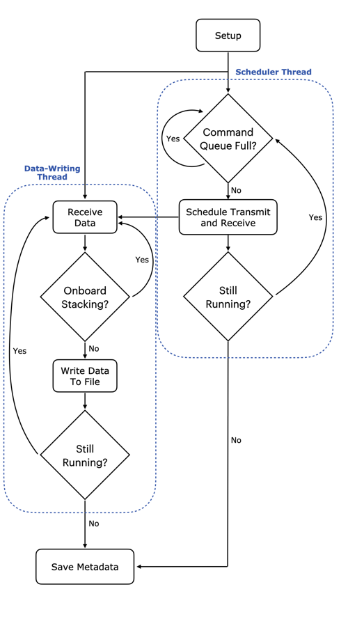
in rf_settings.cpp). The radar code runs in two threads, as shown in the
figure below.
General architecture of the ORCA code
One thread is responsible for scheduling
timed commands
that are enqueued into FIFO queues within the SDR’s FPGA.
The other thead is responsible for pulling received samples from the SDR and
writing them to a file on the host computer.
For a more complete overview, please refer to our paper:
T. O. Teisberg, A. L. Broome and D. M. Schroeder, “Open Radar Code Architecture (ORCA): A Platform for Software-Defined Coherent Chirped Radar Systems,” in IEEE Transactions on Geoscience and Remote Sensing, vol. 62, pp. 1-11, 2024, Art no. 5109411, doi: 10.1109/TGRS.2024.3446368.